Categoría: Solución 2da Eva

Ejercicio: 2Eva_IT2018_T4 Dragado acceso marítimo

a) La matriz para remover sedimentos se determina como la diferencia entre la profundidad y la matriz de batimetría.

Considere el signo de la profundidad para obtener el resultado:

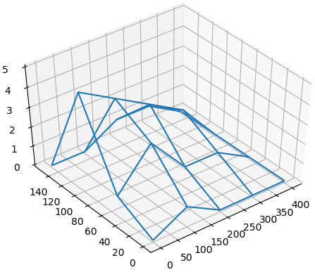
matriz remover sedimentos: 
[[ 4.21  0.    0.96  0.    3.76  3.09]
 [ 2.15  0.11  2.05  3.77  0.    3.07]
 [ 0.    1.14  1.65  0.    1.62  1.35]
 [ 3.7   0.    0.59  2.33  0.    4.23]
 [ 0.    1.38  3.53  4.49  1.98  1.4 ]
 [ 0.    0.77  0.32  1.06  4.24  3.54]]

se obtiene con la instrucciones:

# 2da Evaluación I Término 2018
# Tema 4. canal acceso a Puertos de Guayaquil
import numpy as np

# INGRESO
profcanal = 11

xi = np.array([ 0.,  50., 100., 150., 200., 250.])
yi = np.array([ 0., 100., 200., 300., 400., 500.])

batimetria = [[ -6.79,-12.03,-10.04,-11.60, -7.24,-7.91],
              [ -8.85,-10.89, -8.95, -7.23,-11.42,-7.93],
              [-11.90, -9.86, -9.35,-12.05, -9.38,-9.65],
              [ -7.30,-11.55,-10.41, -8.67,-11.84,-6.77],
              [-12.17, -9.62, -7.47, -6.51, -9.02,-9.60],
              [-11.90,-10.23,-10.68, -9.94, -6.76,-7.46]]

batimetria = np.array(batimetria)
# PROCEDIMIENTO
[n,m] = np.shape(batimetria)

# Matriz remover sedimentos
remover = batimetria + profcanal
for i in range(0,n,1):
    for j in range(0,m,1):
        if remover[i,j]<0:
            remover[i,j]=0
# SALIDA
print('matriz remover sedimentos: ')
print(remover)

b) el volumen se calcula usando el algoritmo de Simpson primero por un eje, y luego con el resultado se continúa con el otro eje,

Considere que existen 6 puntos, o 5 tramos integrar en cada eje.

• Al usar Simpson de 1/3 que usan tramos pares, faltaría integrar el último tramo.
• En el caso de Simpson de 3/8 se requieren tramos multiplos de 3, porl que faltaría un tramo para volver a usar la fórmula.

La solución por filas se implementa usando una combinación de Simpson 3/8 para los puntos entre remover[i, 0:3] y Simpson 1/3 para los puntos entre remover[i, 3:5].

Luego se completa el integral del otro eje con el resultado anterior, aplicando el mismo método.

Se obtuvieron los siguientes resultados:

Integral en eje x: 
[ 219.1   309.83  260.44  217.75  511.21  137.85]
Volumen:  160552.083333

que se obtiene usando las instrucciones a continuación de las anteriores:

# literal b) ---------------------------
def simpson13(fi,h):
    s13 = (h/3)*(fi[0] + 4*fi[1] + fi[2])
    return(s13)
def simpson38(fi,h):
    s38 = (3*h/8)*(fi[0] + 3*fi[1] + 3*fi[2]+ fi[3])
    return(s38)

Integralx = np.zeros(n,dtype = float)

for i in range(0,n,1):
    hx = xi[1]-xi[0]
    fi = remover[i, 0:(0+4)]
    s38 = simpson38(fi,hx)
    fi = remover[i, 3:(3+3)]
    s13 = simpson13(fi,hx)
    Integralx[i] = s38 + s13

hy = yi[1] - yi[0]
fj = Integralx[0:(0+4)]
s38 = simpson38(fj,hy)
fj = Integralx[3:(3+3)]
s13 = simpson13(fj,hy)
volumen = s38 + s13

# Salida
np.set_printoptions(precision=2)
print('Integral en eje x: ')
print(Integralx)
print('Volumen: ', volumen)

Para el examen escrito, se requieren realizar al menos 3 iteraciones/ filas para encontrar el integral.

Ejercicio: 2Eva_IT2018_T1 Paracaidista wingsuit

El problema para un tiempo de observación t>0, se puede dividir en dos partes: velocidad y altura.

1. Determinar velocidad: Se aplica Runge-Kutta con los valores iniciales dados, descartar calcular las alturas.
2. Determinar las altura:  Con los valores de velocidades y la altura inicial de 1 km = 1000 m puede integrar cada tramo.
   Observe las unidades de medida y que la  velocidad es contraria  al eje de altura dy/dt = -v.
3. En el ejercicio se presentan los resultados integrando por trapecios y como otra forma usando la fórmula de Taylor, tomando los puntos encontrados para velocidad.
4. Otra opción para las alturas, en caso de requerir determinar el tiempo exacto en que sucede el resultado es sustituir v = dy/ty y resolver nuevamente la ecuación inicial. (Tarea).

Resultados:

La velocidad máxima, si no hubiese límite en la altura, se encuentra en alrededor de 62.39 m/s.
Sin embargo, luego de 20 segundos se observa que la altura alcanza el valor de cero, es decir se alcanzó tierra con velocidad de  62 m/s, que son algo mas de 223 Km/s, el objeto se estrella…!

altura1 con trapecio, altura2 con Taylor
 [tiempo, velocidad, altura1, altura2]
[[    0.       0.    1000.    1000.  ]
 [    2.      18.64   981.36   980.4 ]
 [    4.      34.04   928.68   925.26]
 [    6.      45.02   849.62   843.37]
 [    8.      52.13   752.47   743.87]
 [   10.      56.49   643.85   633.59]
 [   12.      59.07   528.3    516.97]
 [   14.      60.58   408.65   396.68]
 [   16.      61.45   286.63   274.28]
 [   18.      61.94   163.24   150.66]
 [   20.      62.23    39.07    26.36]
 [   22.      62.39   -85.55   -98.34]]

Los cálculos se realizaron usando las instrucciones en Python:

# 2da Evaluación I Término 2018
# Tema 1. Paracaidista wingsuit
import numpy as np

def rungekutta2(d1y,x0,y0,h,muestras):
    tamano = muestras + 1
    estimado = np.zeros(shape=(tamano,2),dtype=float)
    # incluye el punto [x0,y0]
    estimado[0] = [x0,y0]
    xi = x0
    yi = y0
    for i in range(1,tamano,1):
        K1 = h * d1y(xi,yi)
        K2 = h * d1y(xi+h, yi + K1)

        yi = yi + (K1+K2)/2
        xi = xi + h
        
        estimado[i] = [xi,yi]
    return(estimado)

def integratrapecio(xi,fi,y0):
    tamano = len(xi)
    yi = np.zeros(tamano,dtype = float)
    yi[0] = y0
    for i in range(1,tamano,1):
        h = xi[i]-xi[i-1]
        trapecio = h*(fi[i]+fi[i-1])/2
        yi[i]= yi[i-1] + trapecio
    return(yi)

# PROGRAMA
# INGRESO
g = 9.8
cd = 0.225
m = 90
t0 = 0
v0 = 0

dt = 2
y0 = 1000
muestras = 11

d1v = lambda t,v: g - (cd/m)*(v**2)

# PROCEDIMIENTO
velocidad = rungekutta2(d1v,t0,v0,dt,muestras)
ti = velocidad[:,0]
vi = velocidad[:,1]

# Altura, velocidad es contraria altura,
# integrar en cada tramo por trapecios o Cuadratura de Gauss
altura = integratrapecio(ti,-vi,y0)

# Tabla de resultados
altura = np.transpose([altura])
tabla = np.concatenate((velocidad,altura), axis = 1)

# otra forma: usando Taylor
altura2 = np.zeros(muestras+1,dtype = float)
altura2[0] = y0
for i in range(0, muestras,1):
    acelera = d1v(ti[i],vi[i])
    altura2[i+1] = altura2[i] -(vi[i]*dt + acelera*(dt**2)/2)
# Tabla de resultados
altura2 = np.transpose([altura2])
tabla = np.concatenate((tabla,altura2), axis = 1)

# SALIDA
np.set_printoptions(precision=2)
print('altura1 con trapecio, altura2 con Taylor')
print(' [tiempo, velocidad, altura1,altura2]')
print(tabla)

y para la gráfica:

# Gráfica
import matplotlib.pyplot as plt
plt.subplot(211)
plt.plot(ti,vi,'g')
plt.plot(ti,vi,'bo')
plt.title('paracaidista Wingsuit')
plt.ylabel('velocidad (m/s)')
plt.subplot(212)
plt.plot(ti,altura)
plt.plot(ti,altura,'o')
plt.plot(ti,altura2)
plt.axhline(0, color= 'red')
plt.ylabel('altura (m)')
plt.xlabel('tiempo (s)')
plt.show()

Ejercicio: 2Eva_IIT2017_T4 Problema con valor de frontera

\frac{d^2T}{dx^2} + \frac{1}{x}\frac{dT}{dx} +S =0 0 \leq x \leq 1

Las diferencias finitas a usar son:

\frac{dT}{dx} =\frac{T_{i+1} - T_{i-1}}{2h}+O(h^2) \frac{d^2T}{dx^2}=\frac{T_{i+1} - 2T_i + T_{i-1}}{h^2}+O(h^2)

que al reemplazar el la ecuación:

\frac{T_{i+1} - 2T_i + T_{i-1}}{h^2} + \frac{1}{x_i}\frac{T_{i+1} -T_{i-1}}{2h}+S=0 2x_i (T_{i+1} - 4h x_i T_i + T_{i-1}) + h (T_{i+1} - T_{i-1}) = -2h^2 S x_i T_{i+1}(2x_i + h) - 4x_i T_i + T_{i-1}(2x_i - h) = -2h^2 S x_i T_{i-1}(2x_i - h) - 4x_i T_i + T_{i+1}(2x_i + h)= -2h^2 S x_i

con lo que se puede crear un sistema de ecuaciones para cada valor xi con T₀=2 y T₄ =1 que son parte del enunciado del problema.

Siendo h = 0.25 = 1/4,  y se indica al final que S=1, se crea un sistema de ecuaciones a resolver,

x = [0, 1/4, 1/4, 3/4, 1]

T_{i-1}\Big[2x_i - \frac{1}{4} \Big] - 4x_i T_i + T_{i+1}\Big[2x_i + \frac{1}{4} \Big] = -2\Big(\frac{1}{4}\Big)^2 (1) x_i T_{i-1}\Big[2x_i -\frac{1}{4}\Big] - 4x_i T_i + T_{i+1}\Big[2x_i + \frac{1}{4}\Big] = -\frac{1}{8} x_i

se sustituye con los valores conocidos para cada i:

i=1: 
T0[2(1/4) - 1/4] - 4(1/4)T1 + T2[2(1/4) + 1/4] = -(1/8)(1/4)

     - T1 + (3/4)T2 = -1/32 - (1/4)(2)
     - T1 + (3/4)T2 = -17/32

i=2: 
T1[2(1/2) - 1/4] - 4(1/2)T2 + T3[2(1/2) + 1/4] = -(1/8)(1/2)

     (3/4)T1 - 2T2 + (5/4)T3 = -1/16

i=3: 
T2[2(3/4) - 1/4] - 4(3/4)T3 + T4[2(3/4) + 1/4] = -(1/8)(3/4)

     (5/4)T2 - 3T3 = -3/32 - (7/4)(1)
     (5/4)T2 - 3T3 = -59/32

se ponen las ecuaciones en matrices para resolver con algun metodo numérico:

A = [[ -1, 3/4,   0],
     [3/4,  -2, 5/4],
     [  0, 5/4,  -3]]
B = [-17/32, -1/16, -59/32]
np.linalg.solve(A,B)
array([ 1.54,  1.34,  1.17])

Ejercicio: 2Eva_IIT2017_T1 EDO Runge Kutta 2do Orden d2y/dx2

Tema 1

Runge kutta de 2do Orden
f: y' = z
g: z' = .....
K1y = h f(xi, yi, zi)
K1z = h g(xi, y1, zi)

K2y = h f(xi+h, yi+K1y, zi+K1z)
K2z = h g(xi+h, yi+K1y, zi+K1z)

y(i+1) = yi + (1/2)(K1y + K2y)
z(i+1) = zi + (1/2)(K1z + K2z)

x(i+1) = xi + h
E = O(h3) 
xi ≤ z ≤ x(i+1)

f: z = Θ’
g: z’ = (-gr/L) sin(Θ)

Θ(0) = π/6
z(0) = 0

h=0.1

i=0, t0 = 0, Θ0 = π/6, z0 = 0
    K1y = 0.1(0) = 0
    K1z = 0.1(-9.8/2)sin(π/6) = -0.245

    K2y = 0.1(0+(-0.245)) = -0.0245
    K2z = 0.1(-9.8/2)sin(π/6+0) = -0.245

    Θ1 = π/6 + (1/2)(0+(-0.0245)) = 0.51139
    z1 = 0 + (1/2)(-0.245-0.245) = -0.245
    t1 = 0 + 0.1 = 0.1

i=1, t1 = 0.1, Θ1 = 0.51139, z1 = -0.245
    K1y = 0.1(-0.245) = -0.0245
    K1z = 0.1(-9.8/2)sin(0.51139) = -0.23978

    K2y = 0.1(-0.245+(-0.0245)) = -0.049
    K2z = 0.1(-9.8/2)sin(0.51139+(-0.0245)) = -0.22924

    Θ2 = 0.51139 + (1/2)(-0.0245+(-0.049)) = 0.47509
    z2 = -0.245 + (1/2)(-0.23978+(-0.22924)) = -0.245
    t2 = 0.1 + 0.1 = 0.2

   t         theta     z
[[ 0.        0.523599  0.      ]
 [ 0.1       0.511349 -0.245   ]
 [ 0.2       0.47486  -0.479513]
 [ 0.3       0.415707 -0.692975]
 [ 0.4       0.336515 -0.875098]
 [ 0.5       0.240915 -1.016375]
 [ 0.6       0.133432 -1.108842]
 [ 0.7       0.019289 -1.14696 ]
 [ 0.8      -0.09588  -1.128346]
 [ 0.9      -0.206369 -1.054127]
 [ 1.       -0.306761 -0.92877 ]
 [ 1.1      -0.39224  -0.759461]
 [ 1.2      -0.458821 -0.555246]
 [ 1.3      -0.503495 -0.326207]
 [ 1.4      -0.524294 -0.082851]
 [ 1.5      -0.520315  0.164197]
 [ 1.6      -0.491715  0.404296]
 [ 1.7      -0.439718  0.62682 ]
 [ 1.8      -0.366606  0.821313]
 [ 1.9      -0.275693  0.977893]
 [ 2.       -0.171235  1.087942]]

Literal b), con h= 0.25, con t = 1 ángulo= -0.352484

   t         theta     z
[[ 0.        0.523599  0.      ]
 [ 0.25      0.447036 -0.6125  ]
 [ 0.5       0.227716 -1.054721]
 [ 0.75     -0.070533 -1.170971]
 [ 1.       -0.352484 -0.910162]
 [ 1.25     -0.527161 -0.363031]
 [ 1.5      -0.540884  0.299952]
 [ 1.75     -0.387053  0.890475]
 [ 2.       -0.106636  1.221932]]

El error de del orden h³

---

Instruccciones en python, usando el algoritmo desarrollado en clase

# Runge Kutta de 2do
# EDO de 2do orden con condiciones de inicio
import numpy as np
import matplotlib.pyplot as plt

def rungekutta2_fg(f,g,v0,h,m):
    tabla = [v0]
    xi = v0[0]
    yi = v0[1]
    zi = v0[2]
    for i in range(0,m,1):
        K1y = h * f(xi,yi,zi)
        K1z = h * g(xi,yi,zi)
        
        K2y = h * f(xi+h, yi + K1y, zi+K1z)
        K2z = h * g(xi+h, yi + K1y, zi+K1z)

        yi1 = yi + (1/2)*(K1y+K2y)
        zi1 = zi + (1/2)*(K1z+K2z)
        xi1 = xi + h
        vector = [xi1,yi1,zi1]
        tabla.append(vector)

        xi = xi1
        yi = yi1
        zi = zi1
    tabla = np.array(tabla)
    return(tabla)

# Programa Prueba
# Funciones
f = lambda x,y,z : z
g = lambda x,y,z : (-gr/L)*np.sin(y)

gr = 9.8
L = 2

x0 = 0
y0 = np.pi/6
z0 = 0

v0 = [x0,y0,z0]

h = 0.1
xn = 2
m = int((xn-x0)/h)

# PROCEDIMIENTO
tabla = rungekutta2_fg(f,g,v0,h,m)

xi = tabla[:,0]
yi = tabla[:,1]
zi = tabla[:,2]

# SALIDA
np.set_printoptions(precision=6)
print('x, y, z')
print(tabla)
plt.plot(xi,yi, label='y')
plt.plot(xi,zi, label='z')
plt.legend()
plt.grid()
plt.show()

Ejercicio: 2Eva_IIT2017_T3 EDP parabólica con diferencias regresivas

\frac{dU}{dt} - \frac{1}{16} \frac{d^2U}{dx^2} = 0

Las diferencias finitas requidas en el enunciado son:

U'(x_i,t_j) = \frac{U(x_{i},t_j)-U(x_{i},t_{j-1})}{\Delta t} + O(\Delta t) U''(x_i,t_j) = \frac{U(x_{i+1},t_j)-2U(x_{i},t_j)+U(x_{i-1},t_j)}{\Delta x^2} + O(\Delta x^2)

La indicación de regresiva es para la primera derivada, dependiente de tiempo t.

que al reemplazar en la ecuación sin el término de error, se convierte a.

\frac{U(x_{i},t_j)-U(x_{i},t_{j-1})}{\Delta t} - \frac{1}{16}\frac{U(x_{i+1},t_j)-2U(x_{i},t_j)+U(x_{i-1},t_j)}{\Delta x^2} =0

Se reordenan los términos de forma semejante al modelo planteado en el método básico:

\frac{\Delta t}{16\Delta x^2}[U(x_{i+1},t_j)-2U(x_{i},t_j)+U(x_{i-1},t_j)] = U(x_{i},t_j)-U(x_{i},t_{j-1})

Se simplifica haciendo que haciendo

\lambda = \frac{\Delta t}{16\Delta x^2}

Cambiando la nomenclatura con solo los índices para las variables x y t, ordenando en forma ascendente los índices previo a crear el algoritmo.

\lambda[U(i+1,j)-2U(i,j)+U(i-1,j)] = U(i,j)-U(i,j-1)

Se reordena la ecuación como modelo para el sistema de ecuaciones.

\lambda U(i+1,j)+(-2\lambda-1)U(i,j)+ \lambda U(i-1,j) = -U(i,j-1) P U(i-1,j) + Q U(i,j) + R U(i+1,j) = -U(i,j-1)

Se calculan los valores constantes:

λ = dt/(16*dx2) = 0.05/[16*(1/3)2] = 0.028125

P = λ = 0.028125
Q = (-1-2λ) = (1-2*0.028125) = -1.05625
R = λ = 0.028125

Usando las condiciones del problema:

U(0,t) = U(1,t) = 0, entonces, Ta = 0, Tb = 0

Para los valores de la barra iniciales se debe usar un vector calculado como 2sin(π x) en cada valor de x_i espaciados por hx = 1/3, x entre [0,1]

xi  = [0,1/3, 2/3, 1]
U[xi,0] = [2sin (0*π), 2sin(π/3), 2sin(2π/3), 2sin(π)]
U[xi,0] = [0, 2sin(π/3), 2sin(2π/3), 0]
U[xi,0] = [0, 1.732050,  1.732050, 0]

Con lo que se puede plantear las ecuaciones:

j=1: i=1
0.028125 U(0,1) + (-1.05625) U(1,1) + 0.028125 U(2,1) = -U(1,0)

j=1: i=2
0.028125 U(1,1) + (-1.05625) U(2,1) + 0.028125 U(3,1) = -U(2,0)

y reemplazando los valores de la malla conocidos:

0.028125 (0) – 1.05625 U(1,1) + 0.028125 U(2,1) = -1.732050
0.028125 U(1,1) – 1.05625 U(2,1) + 0.028125 (0) = -1.732050

hay que resolver el sistema de ecuaciones:

-1.05625  U(1,1) + 0.028125 U(2,1) = -1.732050
 0.028125 U(1,1) - 1.05625  U(2,1) = -1.732050

A = [[-1.05625 ,  0.028125],
     [ 0.028125, -1.05625 ]]
B = [-1.732050,-1.732050]
que resuelta con un método numérico:
[ 1.68,  1.68]

Por lo que la solución para una gráfica, con los índices de (fila,columna) como (t,x):

U = [[0, 1.732050,  1.732050, 0],
     [0, 1.680000,  1,680000, 0]]

El error del procedimiento, tal como fué planteado es del orden de O(Δt) y O(Δx²), o error de truncamiento E = O(Δx²) + O(Δt). Δt debe ser menor que Δx en aproximadamente un orden de magnitud

---

Usando algoritmo en python.

Usando lo resuelto en clase y laboratorio, se comprueba la solución con el algoritmo, con hx y ht mas pequeños y más iteraciones:

# EDP parabólicas d2u/dx2  = K du/dt
# método implícito
# Referencia: Chapra 30.3 p.895 pdf.917
#       Rodriguez 10.2.5 p.417
import numpy as np
import matplotlib.pyplot as plt

# INGRESO
# Valores de frontera
Ta = 0
Tb = 0
# longitud en x
a = 0
b = 1
# Constante K
K = 16
# Tamaño de paso
dx = 0.1
dt = 0.01
# temperatura en barra
tempbarra = lambda x: 2*np.sin(np.pi*x)
# iteraciones
n = 100

# PROCEDIMIENTO
# Valores de x
xi = np.arange(a,b+dx,dx)
m = len(xi)

# Resultados en tabla de u
u = np.zeros(shape=(m,n), dtype=float)
# valores iniciales de u
j=0
u[0,j] = Ta
for i in range(1,m-1,1):
    u[i,j] = tempbarra(xi[i])
u[m-1,j] = Tb

# factores P,Q,R
lamb = dt/(K*dx**2)
P = lamb
Q = -1 -2*lamb
R = lamb
vector = np.array([P,Q,R])
tvector = len(vector)

# Calcula U para cada tiempo + dt
j=1
while not(j>=n):
    u[0,j] = Ta
    u[m-1,j] = Tb
    # Matriz de ecuaciones
    tamano = m-2
    A = np.zeros(shape=(tamano,tamano), dtype = float)
    B = np.zeros(tamano, dtype = float)
    for f in range(0,tamano,1):
        for c in range(0,tvector,1):
            c1 = f+c-1
            if(c1>=0 and c1<tamano):
                A[f,c1] = vector[c]
        B[f] = -u[f+1,j-1]
    B[0] = B[0]-P*u[0,j]
    B[tamano-1] = B[tamano-1]-R*u[m-1,j]
    # Resuelve sistema de ecuaciones
    C = np.linalg.solve(A, B) 
    # copia resultados a u[i,j]
    for f in range(0,tamano,1):
        u[f+1,j] = C[f]
    j=j+1 # siguiente iteración
        
# SALIDA
print('Tabla de resultados')
np.set_printoptions(precision=2)
print(u)
# Gráfica
salto = int(n/10)
if (salto == 0):
    salto = 1
for j in range(0,n,salto):
    vector = u[:,j]
    plt.plot(xi,vector)
    plt.plot(xi,vector, '.m')
plt.xlabel('x[i]')
plt.ylabel('t[j]')
plt.title('Solución EDP parabólica')
plt.show()

Ejercicio: 2Eva_IIT2017_T2 Volumen de isla

isla = np.array([[0,1,0,0,0],
                 [1,3,1,1,0],
                 [5,4,3,2,0],
                 [0,0,1,1,0]])

xi = np.array([0,100,200,300,400])
yi = np.array([0, 50,100,150])

Tamaño de la matriz: n=4, m=5

cantidad de elementos por fila impar, aplica Simpson 1/3
hx = (200-0)/2 =100
fila=0
    vector = [0,1,0,0,0]
    deltaA = (100/3)(0+4(1)+0) = 4(100/3)
    deltaA = (100/3)(0+4(0)+0) = 0
    area0 = 4(100/3) + 0 = 4(100/3)
fila=1
    vector = [1,3,1,1,0]
    deltaA = (100/3)(1+4(3)+1) = 14(100/3)
    deltaA = (100/3)(1+4(1)+0) = 5(100/3)
    area1 = 14(100/3) + 5(100/3) = 19(100/3)
fila=2
    vector = [5,4,3,2,0]
    deltaA = (100/3)(5+4(4)+3) = 24(100/3)
    deltaA = (100/3)(3+4(2)+0) = 11(100/3)
    area2 = 24(100/3) + 11(100/3) = 35(100/3)
fila=3
    vector = [0,0,1,1,0]
    deltaA = (100/3)(0+4(0)+1) = (100/3)
    deltaA = (100/3)(1+4(1)+0) = 5(100/3)
    area3 = (100/3) + 5(100/3) = 6(100/3)

areas = [ 4(100/3), 19(100/3), 35(100/3), 6(100/3)]
areas = (100/3)[ 4, 19, 35, 6 ]

areas tiene cantidad de elementos par, aplica Simpson 3/8
    hy = (150-0)/3 = 50
    deltaV = (3/8)(50)(100/3)(4+3(19) + 3(35)+ 6)
           = (25*25)(168)
    Volumen = 107500

tramos:  4 5
areas:  [  133.33333333   633.33333333  1166.66666667    66.66666667]
Volumen:  107500.0

las instrucciones en python para encontrar el valor son:

# 2da Eval II T 2017. Tema 2
# Formula de simpson
# Integración: Regla Simpson 1/3 y 3/8
import numpy as np
import matplotlib.pyplot as plt
from mpl_toolkits.mplot3d import axes3d

def simpson13(xi,yi):
    '''
    las muestras deben ser impares
    '''
    area = 0
    muestras = len(xi)
    impar = muestras%2
    if impar == 1:
        for i in range(0,muestras-2,2):
            h = (xi[i+2] - xi[i])/2
            deltaA = (h/3)*(yi[i]+4*yi[i+1]+yi[i+2])
            area = area + deltaA
    return(area)

def simpson38(xi,yi):
    '''
    las muestras deben ser pares
    '''
    area = 0
    muestras = len(xi)
    impar = muestras%2
    if impar == 0:
        for i in range(0,muestras-3,3):
            h = (xi[i+3] - xi[i])/3
            deltaA = (3*h/8)*(yi[i]+3*yi[i+1]+3*yi[i+2]+yi[i+3])
            area = area + deltaA
    return(area)

def simpson(xi,yi):
    '''
    Selecciona el tipo de algoritmo Simpson
    '''
    muestras = len(xi)
    impar = muestras%2
    if impar == 1:
        area = simpson13(xi,yi)
    else:
        area = simpson38(xi,yi)
    return(area)
    

# INGRESO
isla = np.array([[0,1,0,0,0],
                 [1,3,1,1,0],
                 [5,4,3,2,0],
                 [0,0,1,1,0]])

xi = np.array([0,100,200,300,400])
yi = np.array([0, 50,100,150])

# PROCEDIMIENTO
tamano = np.shape(isla)
n = tamano[0]
m = tamano[1]

areas = np.zeros(n,dtype = float)
for fila in range(0,n,1):
    unafranja = isla[fila,:]
    areas[fila] = simpson(xi,unafranja)
volumen = simpson(yi,areas)

# SALIDA
print('tramos: ', n,m)
print('areas: ', areas)
print('Volumen: ', volumen)

# Gráfica
X, Y = np.meshgrid(xi, yi)
fig = plt.figure()
ax = fig.add_subplot(111, projection = '3d')
ax.plot_wireframe(X,Y,isla)
plt.show()

Ejercicio: 2Eva_IIT2016_T3_MN EDO Taylor 2, Tanque de agua

La solución obtenida se realiza con h=0.5 y usando dos métodos para comparar resultados.

\frac{dy}{dt} = -k \sqrt{y}

1. EDO con Taylor

Usando una aproximación con dos términos de Taylor:

y_{i+1}=y_{i}+ y'_{i} h+\frac{y"_{i}}{2}h^{2}

Por lo que se obtienen las derivadas necesarias:

y'_i= -k (y_i)^{1/2} y"_i= \frac{-k}{2}(y_i)^{-1/2}

1.1 iteraciones

i=0, y₀=3, t₀=0

y'_0= -k(y_0)^{1/2} =-0.06(3)^{1/2} = -0.1039 y"_0= \frac{-0.06}{2}(3)^{-1/2} = -0.0173 y_{1}=y_{0}+ y'_{0} (1)+\frac{y"_{0}}{2}(1)^{2} y_{1}=3+ (-0.1039) (0.5)+\frac{-0.0173}{2}(0.5)^{2}= 2.9458

t₁=t₀+h = 0+0.5= 0.5

i=1, y₁=2.9458, t₁=0.5

y'_1= -k(y_1)^{1/2} =-0.06(2.887)^{1/2} =-0.1029 y"_1= \frac{-0.06}{2}(2.887)^{-1/2} = -0.0174 y_{2}=y_{1}+ y'_{1} (1)+\frac{y"_{1}}{2}(1)^{2} y_{1}=2.9458+ (-0.1029) (1)+\frac{-0.0174}{2}(1)^{2}= 2.8921

t₂=t₁+h = 0.5+0.5 = 1.0

i=2, y₂=2.8921, t₂=1.0

Resolver como Tarea

1.2 Resultados con Python

Realizando una tabla de valores usando Python y una gráfica, encuentra que el valor buscado del tanque a la mitad se obtiene en 16 minutos.

estimado[xi,yi]
[[ 0.          3.        ]
 [ 0.5         2.94587341]
 [ 1.          2.89219791]
 [ 1.5         2.83897347]
 [ 2.          2.7862001 ]
 ...
 [14.          1.65488507]
 [14.5         1.61337731]
 [15.          1.57231935]
 [15.5         1.53171109]
 [16.          1.49155239]
 [16.5         1.45184313]
 [17.          1.41258317]
 [17.5         1.37377234]
 [18.          1.33541049]
 [18.5         1.29749744]
 [19.          1.26003297]
 [19.5         1.22301689]
 [20.          1.18644897]]

Algoritmo en Python para Solución EDO con tres términos:

# EDO. Método de Taylor 3 términos 
# estima la solucion para muestras espaciadas h en eje x
# valores iniciales x0,y0
# entrega arreglo [[x,y]]
import numpy as np

def edo_taylor3t(d1y,d2y,x0,y0,h,muestras):
    tamano = muestras + 1
    estimado = np.zeros(shape=(tamano,2),dtype=float)
    # incluye el punto [x0,y0]
    estimado[0] = [x0,y0]
    x = x0
    y = y0
    for i in range(1,tamano,1):
        y = y + h*d1y(x,y) + ((h**2)/2)*d2y(x,y)
        x = x+h
        estimado[i] = [x,y]
    return(estimado)

# PROGRAMA PRUEBA
# 2Eva_IIT2016_T3_MN EDO Taylor 2, Tanque de agua

# INGRESO.
k=0.06
# d1y = y' = f, d2y = y'' = f'
d1y = lambda x,y: -k*(y**0.5)
d2y = lambda x,y: -(k/2)*(y**(-0.5))
x0 = 0
y0 = 3
h = 1/2
muestras = 40

# PROCEDIMIENTO
puntos = edo_taylor3t(d1y,d2y,x0,y0,h,muestras)
xi = puntos[:,0]
yi = puntos[:,1]

# SALIDA
print('estimado[xi,yi]')
print(puntos)
# Gráfica
import matplotlib.pyplot as plt
plt.plot(xi[0],yi[0],'o', color='r', label ='[x0,y0]')
plt.plot(xi[1:],yi[1:],'o', color='g', label ='y estimada')
plt.axhline(y0/2)
plt.title('EDO: Solución con Taylor 3 términos')
plt.xlabel('x')
plt.ylabel('y')
plt.legend()
plt.grid()
plt.show()

---

2. EDO con Runge-Kutta de 2do Orden dy/dx

Para éste método no se requiere desarrollar la segunda derivada, se usa el mismo h =0.5 con fines de comparación de resultados

2.1 ITeraciones

i = 1, y0=3, t0=0

K_1 = h y'(x_0,y_0) = (0.5)*(-0.06)(3)^{1/2} =-0.05196 K_2 = h y'(x_0+h,y_0+K_1) = (0.5)* y'(0.5,3-0.05196) = -0.05150 y_1 = y_0+\frac{K1+K2}{2} = 3+\frac{-0.05196-0.05150}{2} = 2.9482

i = 2, y1=2.9482, t1=0.5

K_1 = h y'(x_1,y_1) = (0.5)*(-0.06)(2.9482)^{1/2} =-0.05149 K_2 = h y'(x_1+h,y_1+K_1) = (0.5)* y'(0.5,2.9482-0.05149) = -0.05103 y_1 = y_0+\frac{K1+K2}{2} = 3+\frac{-0.05149-0.05103}{2} = -2.8946

i = 3,  y1=2.8946, t1=1.0

Resolver como Tarea

2.2 Resultados con Python

Si comparamos con los resultados anteriores en una tabla, y obteniendo las diferencias entre cada iteración se tiene que:

estimado[xi,yi Taylor, yi Runge-Kutta, diferencias]
[[ 0.0  3.00000000  3.00000000  0.00000000e+00]
 [ 0.5  2.94587341  2.94826446 -2.39104632e-03]
 [ 1.0  2.89219791  2.89697892 -4.78100868e-03]
 [ 1.5  2.83897347  2.84614338 -7.16990106e-03]
 [ 2.0  2.78620010  2.79575783 -9.55773860e-03]
...
 [ 14.0  1.65488507  1.72150488 -6.66198112e-02]
 [ 14.5  1.61337731  1.68236934 -6.89920328e-02]
 [ 15.0  1.57231935  1.64368380 -7.13644510e-02]
 [ 15.5  1.53171109  1.60544826 -7.37371784e-02]
 [ 16.0  1.49155239  1.56766273 -7.61103370e-02]
 [ 16.5  1.45184313  1.53032719 -7.84840585e-02]
 [ 17.0  1.41258317  1.49344165 -8.08584854e-02]
 [ 17.5  1.37377234  1.45700611 -8.32337718e-02]
 [ 18.0  1.33541049  1.42102058 -8.56100848e-02]
 [ 18.5  1.29749744  1.38548504 -8.79876055e-02]
 [ 19.0  1.26003297  1.35039950 -9.03665304e-02]
 [ 19.5  1.22301689  1.31576397 -9.27470733e-02]
 [ 20.0  1.18644897  1.28157843 -9.51294661e-02]]
error en rango:  0.09512946613018003

# EDO. Método de Taylor 3 términos 
# estima la solucion para muestras espaciadas h en eje x
# valores iniciales x0,y0
# entrega arreglo [[x,y]]
import numpy as np

def edo_taylor3t(d1y,d2y,x0,y0,h,muestras):
    tamano = muestras + 1
    estimado = np.zeros(shape=(tamano,2),dtype=float)
    # incluye el punto [x0,y0]
    estimado[0] = [x0,y0]
    x = x0
    y = y0
    for i in range(1,tamano,1):
        y = y + h*d1y(x,y) + ((h**2)/2)*d2y(x,y)
        x = x+h
        estimado[i] = [x,y]
    return(estimado)

def rungekutta2(d1y,x0,y0,h,muestras):
    tamano = muestras + 1
    estimado = np.zeros(shape=(tamano,2),dtype=float)
    # incluye el punto [x0,y0]
    estimado[0] = [x0,y0]
    xi = x0
    yi = y0
    for i in range(1,tamano,1):
        K1 = h * d1y(xi,yi)
        K2 = h * d1y(xi+h, yi + K1)

        yi = yi + (K1+K2)/2
        xi = xi + h
        
        estimado[i] = [xi,yi]
    return(estimado)

# PROGRAMA PRUEBA
# 2Eva_IIT2016_T3_MN EDO Taylor 2, Tanque de agua

# INGRESO.
k=0.06
# d1y = y' = f, d2y = y'' = f'
d1y = lambda x,y: -k*(y**0.5)
d2y = lambda x,y: -(k/2)*(y**(-0.5))
x0 = 0
y0 = 3
h = 1/2
muestras = 40

# PROCEDIMIENTO
puntos = edo_taylor3t(d1y,d2y,x0,y0,h,muestras)
xi = puntos[:,0]
yi = puntos[:,1]

# Con Runge Kutta
puntosRK2 = rungekutta2(d1y,x0,y0,h,muestras)
xiRK2 = puntosRK2[:,0]
yiRK2 = puntosRK2[:,1]

# diferencias
diferencias = yi-yiRK2
error = np.max(np.abs(diferencias))
tabla = np.copy(puntos)
tabla = np.concatenate((puntos,np.transpose([yiRK2]),
                        np.transpose([diferencias])),
                       axis = 1)

# SALIDA
print('estimado[xi,yi Taylor,yi Runge-Kutta,diferencias]')
print(tabla)
print('error en rango: ', error)

# Gráfica
import matplotlib.pyplot as plt
plt.plot(xi[0],yi[0],'o',
         color='r', label ='[x0,y0]')
plt.plot(xi[1:],yi[1:],'o',
         color='g',
         label ='y Taylor 3 terminos')
plt.plot(xiRK2[1:],yiRK2[1:],'o',
         color='blue',
         label ='y Runge-Kutta 2Orden')
plt.axhline(y0/2)
plt.title('EDO: Taylor 3T vs Runge=Kutta 2Orden')
plt.xlabel('x')
plt.ylabel('y')
plt.legend()
plt.grid()
plt.show()

Ejercicio: 2Eva_IT2012_T1_MN Longitud de teleférico

Los datos tomados para el problema son:

x    = [0.00, 0.25, 0.50, 0.75, 1.00]
f(x) = [25.0, 22.0, 32.0, 51.0, 75.0]

Se debe considerar que los datos tienen tamaño de paso (h) del mismo valor.

Literal a)

Fórmulas de orden 2, a partir de:

http://blog.espol.edu.ec/analisisnumerico/formulas-de-diferenciacion-por-diferencias-divididas/

considere que el término del Error O(h²), perdió una unidad del exponente en el proceso, por lo que las fórmulas de orden 2 tienen un error del mismo orden.

Se puede usar por ejemplo:

Para los términos x en el intervalo [0,0.50] hacia adelante

f'(x_i) = \frac{-f(x_{i+2})+4f(x_{i+1})-3f(x_i)}{2h} + O(h^2)

Para el término x con 0.75, centradas:

f'(x_i) = \frac{f(x_{i+1})-f(x_{i-1})}{2h} + O(h^2)

y para el término x con 1.0, hacia atras:

f'(x_i) = \frac{3f(x_{i})-4f(x_{i-1})+f(x_{i-2})}{2h} + O(h^2)

Luego se aplica el resultado en la fórmula:

g(x) = \sqrt{1+[f'(x)]^2}

L = \int_a^b g(x) \delta x .

Literal b)

Use las fórmulas de integración numérica acorde a los intervalos. Evite repetir intervalos, que es el error más común.

Por ejemplo, se puede calcular el integral de g(x) aplicando dos veces Simpson de 1/3, que sería la más fácil de aplicar dado los h iguales.

Otra opción es Simpson de 3/8 añadido un trapecio, otra forma es solo con trapecios en todo el intervalo.

Como ejemplo de cálculo usando un algoritmo en Python se muestra que:

f'(x): [-38.  22.  66.  86. 106.]
 g(x): [ 38.0131  22.0227  66.0075  86.0058 106.0047]
L con S13:  59.01226169578733
L con trapecios:  61.511260218050175

los cálculos fueron realizados a partir de la funciones desarrolladas durante la clase. Por lo que se muestran 3 de ellas en el algoritmo.

import numpy as np
import matplotlib.pyplot as plt

# Funciones para integrar realizadas en clase
def itrapecio (datos,dt):
    n=len(datos)
    integral=0
    for i in range(0,n-1,1):
        area=dt*(datos[i]+datos[i+1])/2
        integral=integral + area 
    return(integral)

def isimpson13(f,h):
    n = len(f)
    integral = 0
    for i in range(0,n-2,2):
        area = (h/3)*(f[i]+4*f[i+1]+f[i+2])
        integral = integral + area
    return(integral)

def isimpson38 (f,h):
    n=len(f)
    integral=0
    for i in range(0,n-3,3):
        area=(3*h/8)*(f[i]+3*f[i+1]+3*f[i+2] +f[i+3] )
        integral=integral + area
    return(integral)

# INGRESO
x = np.array( [0.0,0.25,0.50,0.75,1.00])
fx= np.array([ 25.0, 22.0, 32.0, 51.0, 75.0])

# PROCEDIMIENTO
n = len(fx)
dx = x[1]-x[0]

# Diferenciales
dy = np.zeros(n)

for i in range(0,n-2,1):
    dy[i] = (-fx[i+2]+4*fx[i+1]-3*fx[i])/(2*dx)
# Diferenciales penúltimo
i = n-2
dy[i] = (fx[i+1]-fx[i-1])/(2*dx)
# Diferenciales último
i = n-1
dy[i] = (3*fx[i]-4*fx[i-1]+fx[i-2])/(2*dx)

# Función gx
gx = np.sqrt(1+(dy**2))

# Integral
integral = isimpson13(gx,dx)
integrartr = itrapecio(gx,dx)

# SALIDA 
print('f\'(x):', dy)
print(' g(x):', gx)
print("L con S13: ", integral )
print("L con trapecios: ", integrartr )

plt.plot(x,fx)
plt.show()

La gráfica del cable es:

Ejercicio: 2Eva_IT2012_T2 Modelo de clima

Se deja de tarea realizar las tres primeras iteraciones en papel.

Se presenta el resultado usando el algoritmo de segundo grado como una variante a la respuesta usada como ejemplo.

 [ ti, xi, yi, zi]
[[ 0.0000e+00  1.0000e+01  7.0000e+00  7.0000e+00]
 [ 2.5000e-03  9.9323e+00  7.5033e+00  7.1335e+00]
 [ 5.0000e-03  9.8786e+00  7.9988e+00  7.2774e+00]
 ...
 [ 2.4995e+01 -8.4276e+00 -2.7491e+00  3.3021e+01]
 [ 2.4998e+01 -8.2860e+00 -2.6392e+00  3.2858e+01]
 [ 2.5000e+01 -8.1453e+00 -2.5346e+00  3.2692e+01]]

Algoritmo en Python

# 2Eva_IT2012_T2 Modelo de clima
# MATG1013 Análisis Numérico
import numpy as np
import matplotlib.pyplot as plt

def rungekutta2_fg(f,g,j,t0,x0,y0,z0,h,muestras):
    tamano = muestras + 1
    estimado = np.zeros(shape=(tamano,4),dtype=float)
    # incluye el punto [t0,x0,y0,z0]
    estimado[0] = [t0,x0,y0,z0]
    ti = t0
    xi = x0
    yi = y0
    zi = z0
    for i in range(1,tamano,1):
        K1x = h * f(ti,xi,yi,zi)
        K1y = h * g(ti,xi,yi,zi)
        K1z = h * j(ti,xi,yi,zi)
        
        K2x = h * f(ti+h,xi + K1x, yi + K1y, zi + K1z)
        K2y = h * g(ti+h,xi + K1x, yi + K1y, zi + K1z)
        K2z = h * j(ti+h,xi + K1x, yi + K1y, zi + K1z)
        
        xi = xi + (K1x+K2x)/2
        yi = yi + (K1y+K2y)/2
        zi = zi + (K1z+K2z)/2
        ti = ti + h
        
        estimado[i] = [ti,xi,yi,zi]
    return(estimado)


#INGRESO
to = 0
xo = 10
yo = 7
zo = 7
f = lambda t,x,y,z: 10*(y-x)
g = lambda t,x,y,z: x*(28-z) - y
j = lambda t,x,y,z: -(8/3)*z + (x*y)
h = 0.0025
muestras = 10000

#PROCEDIMIENTO
#Rugen-Kutta 2_orden
tabla = rungekutta2_fg(f,g,j,to,xo,yo,zo,h,muestras)

#SALIDA
np.set_printoptions(precision=4)
print(' [ ti, xi, yi, zi]')
print(tabla)

# Gráfica
from mpl_toolkits.mplot3d import Axes3D
fig = plt.figure()
ax = fig.gca(projection='3d')
ax.plot(tabla[:,1], tabla[:,2], tabla[:,3])
plt.show()

Ejercicio: 2Eva_IIT2011_T3 EDP Parabólica, explícito

La ecuación a resolver es:

\frac{\delta u}{\delta t} - \frac{\delta^2 u}{\delta x^2} =2

Como el método requerido es explícito se usan las diferencias divididas:

\frac{d^2 u}{dx^2} = \frac{u_{i+1,j} - 2 u_{i,j} + u_{i-1,j}}{(\Delta x)^2} \frac{du}{dt} = \frac{u_{i,j+1} - u_{i,j} }{\Delta t}

Reordenando la ecuación al modelo realizado en clase:

\frac{\delta^2 u}{\delta x^2} = \frac{\delta u}{\delta t} - 2 \frac{u_{i+1,j} - 2 u_{i,j} + u_{i-1,j}}{(\Delta x)^2} = \frac{u_{i,j+1} - u_{i,j} }{\Delta t} - 2

multiplicando cada lado por Δt

\frac{\Delta t}{(\Delta x)^2} \Big[u_{i+1,j} - 2 u_{i,j} + u_{i-1,j} \Big]= u_{i,j+1} - u_{i,j} - 2\Delta t

Se establece el valor de

\lambda = \frac{\Delta t}{(\Delta x)^2} \lambda u_{i+1,j} - 2 \lambda u_{i,j} + \lambda u_{i-1,j} = u_{i,j+1} - u_{i,j} - 2\Delta t

obteniendo la ecuación general, ordenada por índices de izquierda a derecha:

\lambda u_{i-1,j} +(1- 2 \lambda)u_{i,j} + \lambda u_{i+1,j} + 2\Delta t = u_{i,j+1}

con valores de:

λ = Δt/(Δx)2 = (0.04)/(0.25)2 = 0.64
P = λ = 0.64
Q = (1-2λ) = -0.28
R = λ = 0.64

0.64 u_{i-1,j} - 0.28 u_{i,j} + 0.64 u_{i+1,j} + 0.08 = u_{i,j+1}

Se realizan 3 iteraciones:

i= 1, j=0

u_{1,1} = 0.64 u_{0,0} -0.28u_{1,0}+0.64 u_{2,0}+0.08 u_{1,1} = 0.64 [\sin(\pi*0)+0*(1-0)]- 0.28[\sin(\pi*0.25)+0.25*(1-0.25)] +0.64[\sin(\pi*0.5)+ 0.5*(1-0.5)]+0.08

u[1,1] =0.89

i = 2, j=0

0.64 u_{1,0} - 0.28 u_{2,0} + 0.64 u_{3,0} + 0.08 = u_{2,1}

u[1,0] = 1.25

i = 3, j=0

0.64 u_{2,0} - 0.28 u_{3,0} + 0.64 u_{4,0} + 0.08 = u_{3,1}

u[3,1] = 0.89

---

Algoritmo en Python

con los valores y ecuación del problema

# EDP parabólicas d2u/dx2  = K du/dt
# método explícito, usando diferencias finitas
# Referencia: Chapra 30.2 p.888 pdf.912
#       Rodriguez 10.2 p.406
import numpy as np
import matplotlib.pyplot as plt

# INGRESO
# Valores de frontera
Ta = 0
Tb = 0
T0 = lambda x: np.sin(np.pi*x)+x*(1-x)
# longitud en x
a = 0
b = 1
# Constante K
K = 1
# Tamaño de paso
dx = 0.1
dt = dx/10/2
# iteraciones en tiempo
n = 50

# PROCEDIMIENTO
# iteraciones en longitud
xi = np.arange(a,b+dx,dx)
m = len(xi)
ultimox = m-1

# Resultados en tabla u[x,t]
u = np.zeros(shape=(m,n), dtype=float)

# valores iniciales de u[:,j]
j=0
ultimot = n-1
u[0,j]= Ta
u[1:ultimox,j] = T0(xi[1:ultimox])
u[ultimox,j] = Tb

# factores P,Q,R
lamb = dt/(K*dx**2)
P = lamb
Q = 1 - 2*lamb
R = lamb

# Calcula U para cada tiempo + dt
j = 0
while not(j>=ultimot):
    u[0,j+1] = Ta
    for i in range(1,ultimox,1):
        u[i,j+1] = P*u[i-1,j] + Q*u[i,j] + R*u[i+1,j]+2*dt
    u[m-1,j+1] = Tb
    j=j+1

# SALIDA
print('Tabla de resultados')
np.set_printoptions(precision=2)
print(u)

# Gráfica
salto = int(n/10)
if (salto == 0):
    salto = 1
for j in range(0,n,salto):
    vector = u[:,j]
    plt.plot(xi,vector)
    plt.plot(xi,vector, '.r')
plt.xlabel('x[i]')
plt.ylabel('t[j]')
plt.title('Solución EDP parabólica')
plt.show()