Ejercicio: 2Eva2010TI_T2 EDO Movimiento angular
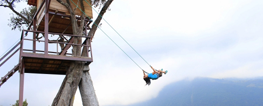
Para resolver, se usa Runge-Kutta_fg de 2do Orden como ejemplo
y'' + 10 \sin (y) =0Para simplificar a primera derivada se plantea:
y' = z = f(t,y,z)convirtiendo la ecuación a:
y'' =z'= -10 \sin (y) = g(t,y,z)teniendo como punto de partida t0=0, y0=0 y z0=0.1
y(0)=0, y'(0)=0.1La tabla inicia como:
| i | ti | yi | vi | K1y | K1v | K2y | K2v | K3y | K3v | K4y | K4v |
|---|---|---|---|---|---|---|---|---|---|---|---|
| 0 | 0 | 0 | 0.1 | - | - | - | - | - | - | - | - |
itera = 0
K1y = 0.1\left( 0.1\right) =0.01 K1v = 0.1\left( -10 \sin (0)\right) =0 K2y = 0.1\left( 0.1+\frac{0}{2}\right) =0.01 K2v = 0.1\left( -10 \sin \left(0+\frac{0.01}{2}\right)\right) =-0.005 K3y = 0.1\left( 0.1+\frac{-0.005}{2}\right) =0.0098 K3v = 0.1\left( -10 \sin \left(0+\frac{0.01}{2}\right)\right) =-0.005 K3y = 0.1\left( 0.1+(-0.005)\right) =0.0095 K4v = 0.1\left( -10 \sin (0+0.0098)\right) =-0.0097 yi = 0+\frac{0.01+2(0.01)+2(0.0098)+0.0095}{6}=0.0098 yi = 0.1+\frac{0+2(-0.005)+2(-0.005)+(-0.0097)}{6}=0.095 ti = 0+0.1 = 0.1| i | ti | yi | vi | K1y | K1v | K2y | K2v | K3y | K3v | K4y | K4v |
|---|---|---|---|---|---|---|---|---|---|---|---|
| 0 | 0 | 0 | 0.1 | - | - | - | - | ||||
| 1 | 0.1 | 0.0098 | 0.095 | 0.01 | 0 | 0.01 | -0.005 | 0.0098 | -0.005 | 0.0095 | -0.0097 |
itera =1
K1y = 0.1\left( 0.095\right) =0.0095 K1v = 0.1\left( -10 \sin (0.0098)\right) =-0.0098 K2y = 0.1\left( 0.095+\frac{-0.0098}{2}\right) =0.009 K2v = 0.1\left( -10 \sin \left(0+\frac{0.0095}{2}\right)\right) =-0.0146...
continua como tarea ..
ti = 0.1+0.1 = 0.2| i | ti | yi | vi | K1y | K1v | K2y | K2v | K3y | K3v | K4y | K4v |
|---|---|---|---|---|---|---|---|---|---|---|---|
| 0 | 0 | 0 | 0.1 | - | - | - | - | ||||
| 1 | 0.1 | 0.0098 | 0.095 | 0.01 | 0 | 0.01 | -0.005 | 0.0098 | -0.005 | 0.0095 | -0.0097 |
| 2 | 0.2 | 0.0187 | 0.0807 | 0.0095 | -0.0098 | 0.009 | -0.0146 | 0.0088 | -0.0143 | 0.0081 | -0.0186 |
Se desarrolla el algoritmo para obtener los valores:
EDO f,g con Runge-Kutta 4 Orden
i  [ xi,  yi,  zi ]
   [ K1y,  K1z,  K2y,  K2z ]
   [ K3y,  K3z,  K4y,  K4z ]
0 [0.  0.  0.1]
  [0. 0. 0. 0.]
  [0. 0. 0. 0.]
1 [0.1    0.0098 0.095 ]
  [ 0.01  -0.     0.01  -0.005]
  [ 0.0098 -0.005   0.0095 -0.0097]
2 [0.2    0.0187 0.0807]
  [ 0.0095 -0.0098  0.009  -0.0146]
  [ 0.0088 -0.0143  0.0081 -0.0186]
3 [0.3    0.0257 0.0583]
  [ 0.0081 -0.0187  0.0071 -0.0227]
  [ 0.0069 -0.0223  0.0058 -0.0256]
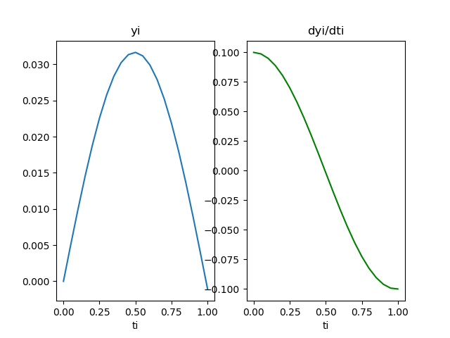
que permiten generar la gráfica de respuesta:
Algoritmo en Python
# 2Eva_IT2010_T2 Movimiento angular
# EDO dy/dx. Metodo de RungeKutta 4to Orden
# estima la solucion para muestras espaciadas h en eje x
# valores iniciales x0,y0
import numpy as np

# INGRESO
f = lambda t,y,v: v
g = lambda t,y,v: -10*np.sin(y)

t0 = 0 # condiciones iniciales
y0 = 0
v0 = 0.1
h  = 0.1
muestras = 20

def rungekutta4_fg(fx,gx,x0,y0,z0,h,muestras,
                   vertabla=False, precision=6):
    ''' solucion a EDO d2y/dx2 con Runge-Kutta 4to Orden,
    f(x,y,z) = z #= y'
    g(x,y,z) = expresion d2y/dx2 con z=y'
    tambien es solucion a sistemas edo f() y g()
    x0,y0,z0 son valores iniciales, h es tamano de paso,
    muestras es la cantidad de puntos a calcular.
    '''
    tamano = muestras + 1
    tabla = np.zeros(shape=(tamano,3+8),dtype=float)
    # incluye el punto [x0,y0]
    tabla[0] = [x0,y0,z0,0,0,0,0,0,0,0,0]

    xi = x0 # valores iniciales
    yi = y0
    zi = z0
    for i in range(1,tamano,1):
        K1y = h * fx(xi,yi,zi)
        K1z = h * gx(xi,yi,zi)

        K2y = h * fx(xi+h/2, yi + K1y/2, zi + K1z/2)
        K2z = h * gx(xi+h/2, yi + K1y/2, zi + K1z/2)

        K3y = h * fx(xi+h/2, yi + K2y/2, zi + K2z/2)
        K3z = h * gx(xi+h/2, yi + K2y/2, zi + K2z/2)

        K4y = h * fx(xi+h, yi + K3y, zi + K3z)
        K4z = h * gx(xi+h, yi + K3y, zi + K3z)

        yi = yi + (K1y+2*K2y+2*K3y+K4y)/6
        zi = zi + (K1z+2*K2z+2*K3z+K4z)/6
        xi = xi + h

        tabla[i] = [xi,yi,zi,K1y,K1z,K2y,K2z,K3y,K3z,K4y,K4z]

    if vertabla==True:
        np.set_printoptions(precision)
        print('EDO f,g con Runge-Kutta 4 Orden')
        print('i ','[ xi,  yi,  zi',']')
        print('   [ K1y,  K1z,  K2y,  K2z ]')
        print('   [ K3y,  K3z,  K4y,  K4z ]')
        for i in range(0,tamano,1):
            txt = ' '
            if i>=10:
                txt = '  '
            print(str(i),tabla[i,0:3])
            print(txt,tabla[i,3:7])
            print(txt,tabla[i,7:])

    return(tabla)
# PROCEDIMIENTO
tabla = rungekutta4_fg(f,g,t0,y0,v0,h,muestras,
                       vertabla=True, precision=4)
# SALIDA
# print('tabla de resultados')
# print(tabla)

# GRAFICA ---------------------
import matplotlib.pyplot as plt

titulo = 'EDO Runge-Kutta 2ord - Movimiento angular'
etiq_x = 't = tiempo'
etiq_y = 'y = altura'
etiq_z = 'v = velocidad'

i = muestras # iteración en gráfica

titulo = titulo+', i='+str(i)
xi = tabla[:,0]
yi = tabla[:,1]
zi = tabla[:,2]
K1y = tabla[:,3]
K1z = tabla[:,4]
K2y = tabla[:,5]
K2z = tabla[:,6]

plt.subplot(211)
plt.plot(xi[0],yi[0],'o',
         color='red', label ='[t0,y0]')
plt.plot(xi[1:i+2],yi[1:i+2],'o',
         color='green', label ='[t[i],y[i]]')
plt.plot(xi[0:i+2],yi[0:i+2],
         color='blue',label='y(t)')
if i<muestras: # gráfica para una iteración
    plt.plot(xi[i+1],yi[i+1],'o',color='orange',
             label ='[x[i+1],y[i+1]]')
    plt.plot(xi[i:i+3],yi[i:i+3],'.',color='gray')
    plt.plot(xi[i:i+2],[yi[i],yi[i]], color='orange',
             label='h',linestyle='dashed')
    plt.plot([xi[i+1]-0.02*h,xi[i+1]-0.02*h],
             [yi[i],yi[i]+K1y[i+1]],
             color='green',label='K1y',linestyle='dashed')
    plt.plot([xi[i+1]+0.02*h,xi[i+1]+0.02*h],
             [yi[i],yi[i]+K2y[i+1]],
             color='magenta',label='K2y',linestyle='dashed')
    plt.plot([xi[i+1]-0.02*h,xi[i+1]+0.02*h],
             [yi[i]+K1y[i+1],yi[i]+K2y[i+1]],
             color='magenta')
if np.min(yi[0:i+1])<0: # linea 0
    plt.axhline(0, color='red')
plt.ylabel(etiq_y)
plt.legend()
plt.grid()
plt.tight_layout()

plt.subplot(212)
plt.plot(xi[0],zi[0],'o',
         color='red', label ='[t0,v0]')
plt.plot(xi[1:i+2],zi[1:i+2],'o',
         color='green', label ='[t[i],v[i]]')
plt.plot(xi[0:i+2],zi[0:i+2],
         color='green',label='v(t)')
if i<muestras: # gráfica para una iteración
    plt.plot(xi[i+1],zi[i+1],'o',color='orange',
             label ='[t[i+1],v[i+1]]')
    plt.plot(xi[i:i+3],zi[i:i+3],'.',color='gray')
    plt.plot(xi[i:i+2],[zi[i],zi[i]], color='orange',
             label='h',linestyle='dashed')
    plt.plot([xi[i+1]-0.02*h,xi[i+1]-0.02*h],
             [zi[i],zi[i]+K1z[i+1]],
             color='green',label='K1z',linestyle='dashed')
    plt.plot([xi[i+1]+0.02*h,xi[i+1]+0.02*h],
             [zi[i],zi[i]+K2z[i+1]],
             color='magenta',label='K2z',linestyle='dashed')
    plt.plot([xi[i+1]-0.02*h,xi[i+1]+0.02*h],
             [zi[i]+K1z[i+1],zi[i]+K2z[i+1]],
             color='magenta')

plt.suptitle(titulo)
plt.xlabel(etiq_x)
plt.ylabel(etiq_z)
plt.legend()
plt.grid()
plt.tight_layout()

plt.show() #comentar para la siguiente gráfica