Ejercicio: 2Eva2022PAOII_T2 EDO - población de protestantes en una sociedad
El sistema de ecuaciones para el ejercicio se expresa como:
\frac{\delta}{\delta t}x(t) = b x(t) - d (x(t))^2 \frac{\delta}{\delta t}y(t) = b y(t) - d (y(t))^2 +r b (x(t)-y(t))literal a
Simplificando la nomenclatura, la población total del país se describe con:
x' = b x - d x^2La población de protestantes se describe con;
y' = b y - d y^2 +r b (x-y)Sustituyendo constantes, y considerando x(0)=1 ; y(0)=0.01 ; h=0.5 valores del enunciado:
x' = 0.02 x - 0.015 x^2 y' = 0.02 y - 0.015 y^2 +0.1(0.02) (x-y)El planteamiento de Runge-Kutta se hace junto a la primera iteración, además de encontrarse en las instrucciones con Python.
literal b
Se describen 3 iteraciones usando los resultados de la tabla con el algoritmo, para mostrar la comprensión del algoritmo.
| i | ti | xi | yi |
|---|---|---|---|
| 0 | 0 | 1 | 0.01 |
t = 0 para iniciar las iteraciones, h=0.5
K1x = 0.5 \left(0.02 (1) - 0.015 (1)^2 \right) = 0.0025 K1y = 0.5\left(0.02 (0.01) - 0.015 (0.01)^2 +0.1(0.02) (1-0.01)\right) = 0.001089.
K2x = 0.5 \left(0.02 (1+0.0025) - 0.015 (1+0.0025)^2 \right) = 0.00248 K2y = 0.5\Big(0.02 (0.01+0.00108) - 0.015 (0.01+0.00108)^2 + 0.1(0.02) ((1+0.0025)-(0.01+0.00108))\Big) = 0.001101La población del país en la iteración se actualiza a:
x_1 = 1 + \frac{0.0025+0.00248}{2} = 1.0025La población de protestantes en la iteración se actualiza a:
y_1 = 0.01 + \frac{0.001089+0.001101}{2} = 0.01109t1 = 0 + 0.5 =0.5
Se actualiza la tabla con los valores obtenidos:
| i | ti | xi | yi |
|---|---|---|---|
| 0 | 0 | 1 | 0.01 |
| 1 | 0.5 | 1.0025 | 0.01109 |
t=0.5
K1x = 0.5 \left( 0.02 (1.0025) - 0.015 (1.0025)^2 \right)= 0.002487 K1y = 0.5\left( 0.02 (0.01109) - 0.015 (0.01109)^2 +0.1(0.02) (1.0025-0.01109)\right)= 0.001101.
K2x = 0.5 \left(0.02 (1.0025+ 0.002487) - 0.015 (1.0025+ 0.002487)^2 \right) = 0.002474 K2y = 0.5 \Big( 0.02 (0.01109+0.001101) - 0.015(0.01109+0.001101)^2 + 0.1(0.02)((1.0025+ 0.002487)-(0.01109+0.001101))\Big) = 0.001113.
x_2 = 1.0025 + \frac{0.002487+0.002474}{2} = 1.0050 y_2 = 0.01109 + \frac{0.001101+0.001113}{2} = 0.01220t2 = 0.5 + 0.5 = 1
| i | ti | xi | yi |
|---|---|---|---|
| 0 | 0 | 1 | 0.01 |
| 1 | 0.5 | 1.0025 | 0.01109 |
| 2 | 1 | 1.0050 | 0.01220 |
t=1
K1x = 0.5 \left( 0.02 (1.0050) - 0.015 (1.0050)^2 \right)= 0.002474 K1y = 0.5 \left(0.02 (0.01220) - 0.015 (0.01220)^2 +0.1(0.02) (1.0050-0.01220) \right)= 0.001113.
K2x = 0.5 \left(0.02 (1.0050+ 0.002474) - 0.015 (1.0050+ 0.002474)^2 \right) = 0.002462 K2y = 0.5 \Big(0.02 (0.01220+0.001113) - 0.015 (0.01220+0.001113)^2 + 0.1(0.02) ((1.0050+ 0.002474)-(0.01220+0.001113))\Big) = 0.001126.
x_3 = 1.0050 + \frac{0.002474+0.002462}{2} = 1.0074 y_3 = 0.01220 + \frac{0.001113+0.001126}{2} = 0.01332t3 = 1 + 0.5 = 1.5
| i | ti | xi | yi |
|---|---|---|---|
| 0 | 0 | 1 | 0.01 |
| 1 | 0.5 | 1.0025 | 0.01109 |
| 2 | 1 | 1.0050 | 0.01220 |
| 3 | 1.5 | 1.0074 | 0.01332 |
Resultado con el algoritmo
Para obtener los datos de las iteraciones, primero se ejecuta el algoritmo para pocas iteraciones.
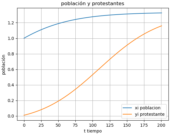
Para la pregunta sobre 200 años, se incrementa las iteraciones a 2 por año y las condiciones iniciales, es decir 401 muestras.
 EDO f,g con Runge-Kutta 2 Orden
i  [ xi,  yi,  zi ]
   [ K1y,  K1z,  K2y,  K2z ]
0 [0.   1.   0.01]
  [0. 0. 0. 0.]
1 [0.5      1.002494 0.011095]
  [0.0025   0.001089 0.002487 0.001101]
2 [1.       1.004975 0.012203]
  [0.002487 0.001101 0.002475 0.001114]
3 [1.5      1.007444 0.013323]
  [0.002475 0.001114 0.002462 0.001126]
4 [2.       1.0099   0.014455]
  [0.002462 0.001126 0.00245  0.001138]
5 [2.5      1.012343 0.0156  ]
  [0.00245  0.001138 0.002437 0.001151]
6 [3.       1.014774 0.016757]
  [0.002437 0.001151 0.002424 0.001163]
7 [3.5      1.017192 0.017926]
  [0.002424 0.001163 0.002412 0.001176]
8 [4.       1.019597 0.019109]
  [0.002412 0.001176 0.002399 0.001189]
9 [4.5      1.02199  0.020304]
  [0.002399 0.001189 0.002386 0.001202]
10 [5.       1.02437  0.021512]
   [0.002386 0.001202 0.002374 0.001214]
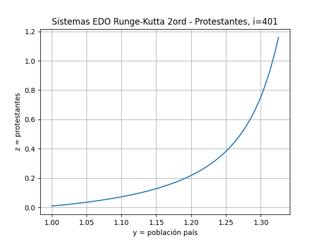
...Observación: La población identificada como protestante, continua creciendo, mientras que la proporción de "conformistas" se reduce según los parámetros indicados en el ejercicio. Los valores de natalidad y defunción cambian con el tiempo mucho más en años por otras variables, por lo que se deben realizar ajustes si se pretende extender el modelo.
Algoritmo en Python
# Modelo predador-presa de Lotka-Volterra
# 2Eva2022PAOII_T2 EDO - población de protestantes en una sociedad
# Sistemas EDO con Runge Kutta de 2do Orden
import numpy as np

# INGRESO
# Parámetros de las ecuaciones
b = 0.02
d = 0.015
r = 0.1

# Ecuaciones
f = lambda t,x,y : (b-d*x)*x
g = lambda t,x,y : (b-d*y)*y + r*b*(x-y)

# Condiciones iniciales
t0 = 0
x0 = 1
y0 = 0.01

# parámetros del algoritmo
h = 0.5
muestras = 401

# Algoritmo como función
def rungekutta2_fg(f,g,x0,y0,z0,h,muestras,
                   vertabla=False, precision=6):
    ''' solucion a EDO d2y/dx2 con Runge-Kutta 2do Orden,
    f(x,y,z) = z #= y'
    g(x,y,z) = expresion d2y/dx2 con z=y'
    tambien es solucion a sistemas edo f() y g()
    x0,y0,z0 son valores iniciales, h es tamano de paso,
    muestras es la cantidad de puntos a calcular.
    '''
    tamano = muestras + 1
    tabla = np.zeros(shape=(tamano,3+4),dtype=float)
    # incluye el punto [x0,y0,z0,K1y,K1z,K2y,K2z]
    tabla[0] = [x0,y0,z0,0,0,0,0]

    xi = x0 # valores iniciales
    yi = y0
    zi = z0
    for i in range(1,tamano,1):
        K1y = h * f(xi,yi,zi)
        K1z = h * g(xi,yi,zi)

        K2y = h * f(xi+h, yi + K1y, zi + K1z)
        K2z = h * g(xi+h, yi + K1y, zi + K1z)

        yi = yi + (K1y+K2y)/2
        zi = zi + (K1z+K2z)/2
        xi = xi + h

        tabla[i] = [xi,yi,zi,K1y,K1z,K2y,K2z]

    if vertabla==True:
        np.set_printoptions(precision)
        print('EDO f,g con Runge-Kutta 2 Orden')
        print('i ','[ xi,  yi,  zi',']')
        print('   [ K1y,  K1z,  K2y,  K2z ]')
        for i in range(0,tamano,1):
            txt = ' '
            if i>=10:
                txt = '  '
            print(str(i),tabla[i,0:3])
            print(txt,tabla[i,3:])

    return(tabla)

# PROCEDIMIENTO
tabla = rungekutta2_fg(f,g,t0,x0,y0,h,
                       muestras,vertabla=True)
# SALIDA
print('Sistemas EDO RK2')
##print('i ','[ xi,  yi,  zi',']')
##print('   [ K1y,  K1z,  K2y,  K2z ]')
##for i in range(0,tamano,1):
##    txt = ' '
##    if i>=10:
##        txt = '  '
##    print(str(i),tabla[i,0:3])
##    print(txt,tabla[i,3:])
Instrucciones para la parte gráfica
# GRAFICA ---------------------
import matplotlib.pyplot as plt

titulo = 'Sistemas EDO Runge-Kutta 2ord - Protestantes'
etiq_x = 'x = tiempo'
etiq_y = 'y = población país'
etiq_z = 'z = protestantes'
i = muestras # iteración en gráfica

titulo = titulo+', i='+str(i)
xi = tabla[:,0]
yi = tabla[:,1]
zi = tabla[:,2]
K1y = tabla[:,3]
K1z = tabla[:,4]
K2y = tabla[:,5]
K2z = tabla[:,6]

plt.subplot(211)
plt.plot(xi[0],yi[0],'o',
         color='red', label ='[t0,y0]')
if i<20: # evita muchos puntos
    plt.plot(xi[1:i+2],yi[1:i+2],'o',
             color='green', label ='[t[i],y[i]]')
plt.plot(xi[0:i+2],yi[0:i+2],
         color='blue',label='y(t)')
if i<muestras: # gráfica para una iteración
    plt.plot(xi[i+1],yi[i+1],'o',color='orange',
             label ='[x[i+1],y[i+1]]')
    plt.plot(xi[i:i+3],yi[i:i+3],'.',color='gray')
    plt.plot(xi[i:i+2],[yi[i],yi[i]], color='orange',
             label='h',linestyle='dashed')
    plt.plot([xi[i+1]-0.02*h,xi[i+1]-0.02*h],
             [yi[i],yi[i]+K1y[i+1]],
             color='green',label='K1y',linestyle='dashed')
    plt.plot([xi[i+1]+0.02*h,xi[i+1]+0.02*h],
             [yi[i],yi[i]+K2y[i+1]],
             color='magenta',label='K2y',linestyle='dashed')
    plt.plot([xi[i+1]-0.02*h,xi[i+1]+0.02*h],
             [yi[i]+K1y[i+1],yi[i]+K2y[i+1]],
             color='magenta')
if np.min(yi[0:i+1])<0: # linea 0
    plt.axhline(0, color='red')
plt.ylabel(etiq_y)
plt.title(titulo)
plt.legend()
plt.grid()
plt.tight_layout()

plt.subplot(212)
plt.plot(xi[0],zi[0],'o',
         color='red', label ='[t0,z0]')
if i<20: # evita muchos puntos
    plt.plot(xi[1:i+2],zi[1:i+2],'o',
             color='green', label ='[t[i],v[i]]')
plt.plot(xi[0:i+2],zi[0:i+2],
         color='green',label='z(t)')
if i<muestras: # gráfica para una iteración
    plt.plot(xi[i+1],zi[i+1],'o',color='orange',
             label ='[t[i+1],z[i+1]]')
    plt.plot(xi[i:i+3],zi[i:i+3],'.',color='gray')
    plt.plot(xi[i:i+2],[zi[i],zi[i]], color='orange',
             label='h',linestyle='dashed')
    plt.plot([xi[i+1]-0.02*h,xi[i+1]-0.02*h],
             [zi[i],zi[i]+K1z[i+1]],
             color='green',label='K1z',linestyle='dashed')
    plt.plot([xi[i+1]+0.02*h,xi[i+1]+0.02*h],
             [zi[i],zi[i]+K2z[i+1]],
             color='magenta',label='K2z',linestyle='dashed')
    plt.plot([xi[i+1]-0.02*h,xi[i+1]+0.02*h],
             [zi[i]+K1z[i+1],zi[i]+K2z[i+1]],
             color='magenta')

plt.xlabel(etiq_x)
plt.ylabel(etiq_z)
plt.legend()
plt.grid()
plt.tight_layout()

#plt.show() #comentar para la siguiente gráfica

# gráfica yi vs zi
fig_yz, graf3 = plt.subplots()
graf3.plot(yi,zi)

graf3.set_title(titulo)
graf3.set_xlabel(etiq_y)
graf3.set_ylabel(etiq_z)
graf3.grid()
plt.show() #comentar para la siguiente gráfica