Ejercicio: 2Eva2025PAOII_T2 EDO trayectoria avión de papel
Los valores iniciales para el ejercicio se consideran como: g=9.8 m/s2, t0 = 0, v0=4, ω0 =0, x0=0, y0=2
literal a
Se indica que el planteamiento es para v(t), ω(t). En el literal b se indica el tamaño de paso h=0.1
f(t,v,\omega) = -0.1388 v^2 - 9.8 \sin(\omega) g(t,v,\omega) = \frac{0.7654 v^2 - 9.8 \cos(\omega)}{v}Usando Runge-Kutta de 2do orden para sistemas de ecuaciones:
K1v = h f(t,v,\omega) = 0.1 (-0.1388 v^2 - 9.8 \sin(\omega)) K1\omega = h g(t,v,\omega) = 0.1 \frac{0.7654 v^2 - 9.8 \cos(\omega)}{v} K2v = h f(t+h,v+K1v,\omega+K1\omega) = 0.1 (-0.1388 (v+K1v)^2 - 9.8 \sin(\omega+K1\omega) K2\omega = h g(t+h,v+K1v,\omega+K1\omega) = 0.1 \frac{0.7654 (v+K1v)^2 - 9.8 \cos(\omega+K1\omega)}{v+K1v} v[i+1] = v[i] + \frac{K1v+K2v}{2} \omega[i+1] = \omega[i] + \frac{K1\omega+K2\omega}{2} t[i+1] =t[i] + hliteral b
iteración = 0, t0 = 0, v0=4, ω0 =0
Usando Runge-Kutta de 2do orden para sistemas de ecuaciones:
K1v = 0.1 (-0.1388 (4)^2 - 9.8\sin(0)) =-0.2220 K1\omega = 0.1 \frac{0.7654 (4)^2 - 9.8 \cos(0)}{4} =0.26116 K2v = 0.1 (-0.1388 (4-0.2220)^2 - 9.8 \sin(0+0.26116)) =-0.258004 K2\omega = 0.1 \frac{0.7654 (4-0.2220)^2 - 9.8 \cos(0+0.26116)}{4-0.2220} =0.03024 v[1] = 4 + \frac{-0.2220-0.258004}{2} =3.7599 \omega[1] = 0 + \frac{0.26116+0.03024}{2} =0.04570 t[1] =0 + 0.1 = 0.1iteración = 1, t0 = 0.1, v0=3.7599, ω0 =0.04570
K1v = 0.1 (-0.1388 (3.7599)^2 - 9.8\sin(0.04570)) =-0.2409 K1\omega = 0.1 \frac{0.7654 (3.7599)^2 - 9.8 \cos(0.04570)}{3.7599} =0.02741 K2v = 0.1 (-0.1388 (3.7599-0.2409)^2 - 9.8 \sin(0.04570+0.02741) =-0.2434 K2\omega = 0.1 \frac{0.7654 (3.7599-0.2409)^2 - 9.8 \cos(0.04570+0.02741)}{3.7599-0.2409}=-0.008406 v[2] = 3.7599 + \frac{-0.2409-0.2434}{2} =3.5177 \omega[2] = 0.04570 + \frac{0.02741-0.008406}{2}=0.05520 t[2] =0.1 + 0.1 =0.2iteración = 2, t0 = 0.2, v0=3.5177, ω0 =0.05520
K1v = 0.1 (-0.1388 (3.5177)^2 - 9.8 \sin(0.05520 )) =-0.2258 K1\omega = 0.1 \frac{0.7654 (3.5177)^2 - 9.8 \cos(0.05520 )}{3.5177} =-0.1957 K2v = 0.1 (-0.1388 (3.5177-0.2258)^2 - 9.8 \sin(0.05520 -0.1957) =-0.008918 K2\omega = 0.1 \frac{0.7654 (3.5177-0.2258)^2 - 9.8 \cos(0.05520 -0.1957)}{3.5177-0.2258} =-0.04542 v[3] = 3.5177 + \frac{-0.2258-0.008918}{2} \omega[3] = 0.05520 + \frac{-0.1957-0.04542}{2} t[3] =0.2 + 0.1 = 0.3literal c
usando el algoritmo:
i  [ xi,  yi,  zi ]
   [ K1y,  K1z,  K2y,  K2z ]
0 [0. 4. 0.]
  [0. 0. 0. 0.]
1 [0.1      3.759908 0.045703]
  [-0.222133  0.061164 -0.25805   0.030241]
2 [0.2      3.517638 0.055201]
  [-0.24104   0.027415 -0.2435   -0.008417]
3 [0.3      3.306824 0.028019]
  [-0.225859 -0.008928 -0.195769 -0.045437]
4 [ 0.4       3.156694 -0.030508]
  [-0.179271 -0.043133 -0.12099  -0.073922]
5 [ 0.5       3.086496 -0.108154]
  [-0.10845  -0.06869  -0.031945 -0.0866  ]
6 [ 0.6       3.099629 -0.188073]
  [-0.026475 -0.079413  0.05274  -0.080425]
7 [ 0.7       3.182333 -0.254509]
  [ 0.04984  -0.073343  0.115569 -0.059528]
8 [ 0.8       3.309327 -0.297833]
  [ 0.106135 -0.054451  0.147852 -0.032198]
...
35 [ 3.5       3.526395 -0.162191]
   [-0.019245 -0.001804 -0.015611 -0.004688]
36 [ 3.6       3.514804 -0.167548]
   [-0.014394 -0.004343 -0.008789 -0.006371]
37 [ 3.7       3.50996  -0.173924]
   [-0.008082 -0.00589  -0.001606 -0.006863]
38 [ 3.8       3.511635 -0.180218]
   [-0.001452 -0.006337  0.004803 -0.00625 ]
39 [ 3.9       3.518653 -0.185496]
   [ 0.004456 -0.005769  0.00958  -0.004787]
40 [ 4.        3.529203 -0.189115]
   [ 0.008857 -0.004416  0.012243 -0.002822]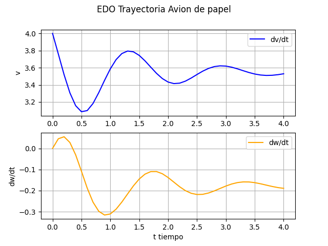
literal d
Se observa que la velocidad y el ángulo oscilan en la trayectoria del avión durante el descenso, lo que se muestra en la gráfica de trayectoria del tema 1.
El algoritmo permite realizar el cálculo con otros valores de velocidad inicial y ángulo w.
El desarrollo presentado debe limitarse hasta cuando se toca el suelo en y=0, esto se logra determinar al incorporar al ejercicio las cuatro ecuaciones del modelo presentado o usando integración para x, y a partir de velocidad y ángulo desde el punto de partida.
Algoritmo en Python
# 2Eva2025PAOII_T2 EDO trayectoria avión de papel v,w
# Sistemas EDO con Runge Kutta de 2do Orden
import numpy as np

def rungekutta2_fg(f,g,x0,y0,z0,h,muestras,
                   vertabla=False, precision=6):
    ''' solucion a EDO d2y/dx2 con Runge-Kutta 2do Orden,
    f(x,y,z) = z #= y'
    g(x,y,z) = expresion d2y/dx2 con z=y'
    tambien es solucion a sistemas edo f() y g()
    x0,y0,z0 son valores iniciales, h es tamano de paso,
    muestras es la cantidad de puntos a calcular.
    '''
    tamano = muestras + 1
    tabla = np.zeros(shape=(tamano,3+4),dtype=float)
    # incluye el punto [x0,y0,z0,K1y,K1z,K2y,K2z]
    tabla[0] = [x0,y0,z0,0,0,0,0]

    xi = x0 # valores iniciales
    yi = y0
    zi = z0
    for i in range(1,tamano,1):
        K1y = h * f(xi,yi,zi)
        K1z = h * g(xi,yi,zi)

        K2y = h * f(xi+h, yi + K1y, zi + K1z)
        K2z = h * g(xi+h, yi + K1y, zi + K1z)

        yi = yi + (K1y+K2y)/2
        zi = zi + (K1z+K2z)/2
        xi = xi + h

        tabla[i] = [xi,yi,zi,K1y,K1z,K2y,K2z]

    if vertabla==True:
        np.set_printoptions(precision)
        print('EDO f,g con Runge-Kutta 2 Orden')
        print('i ','[ xi,  yi,  zi',']')
        print('   [ K1y,  K1z,  K2y,  K2z ]')
        for i in range(0,tamano,1):
            txt = ' '
            if i>=10:
                txt = '  '
            print(str(i),tabla[i,0:3])
            print(txt,tabla[i,3:])

    return(tabla)

# PROGRAMA ------------------

# INGRESO
# Ecuaciones
f = lambda t,v,w: -0.1388*(v**2) - 9.8*np.sin(w)
g = lambda t,v,w: (0.7654*(v**2) - 9.8*np.cos(w))/v

# Condiciones iniciales
t0 = 0. #tiempo
v0 = 4.0 # velocidad
w0 = 0. # ángulo

# parámetros del algoritmo
h = 0.1
muestras = 40

# PROCEDIMIENTO
tabla = rungekutta2_fg(f,g,t0,v0,w0,h,muestras,vertabla=True)
ti = tabla[:,0]
xi = tabla[:,1]
yi = tabla[:,2]

# SALIDA
print('Sistemas EDO: Trayectoria avion de papel')
np.set_printoptions(precision=6)
print(' [ ti, vi, wi,K1v,K1w,K2v,K2w]')
print(tabla[:,0:7])

# GRAFICA tiempos vs población
import matplotlib.pyplot as plt

fig_t, (graf1,graf2) = plt.subplots(2)
fig_t.suptitle('EDO Trayectoria Avion de papel')
graf1.plot(ti,xi, color='blue',label='dv/dt')

#graf1.set_xlabel('t tiempo')
graf1.set_ylabel('v')
graf1.legend()
graf1.grid()

graf2.plot(ti,yi, color='orange',label='dw/dt')
graf2.set_xlabel('t tiempo')
graf2.set_ylabel('dw/dt')
graf2.legend()
graf2.grid()

# gráfica xi vs yi
fig_xy, graf3 = plt.subplots()
graf3.plot(xi,yi)

graf3.set_title('EDO Trayectoria Avion de papel')
graf3.set_xlabel('v')
graf3.set_ylabel('w')
graf3.grid()
plt.show()