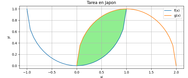
s2Eva2025PAOII_T3 Área en forma de almendra

Ejercicio: 2Eva2025PAOII_T3 Área en forma de almendra

A partir de las expresiones que corresponden a círculos, se encuentra el valor de y:

f(x): (x-0)² +(y-1)² = 1² ; centrado en [0,1]

g(x): (x-1)² +(y-0)² = 1² ; centrado en [1,0]

literal a.

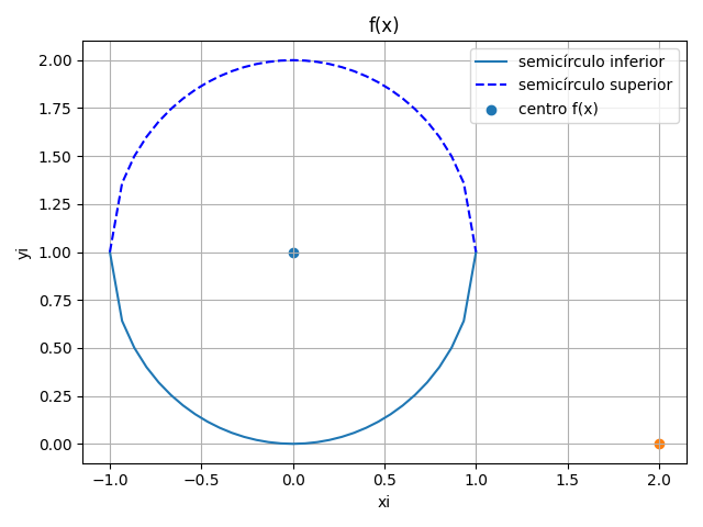
El primer semicírculo se obtiene de f(x): (x-0)² +(y-1)² = 1²

(y-1)² = 1² - (x-0)²

y-1 = \pm \sqrt{ 1 - (x-0)^2}

y =1 \pm \sqrt{ 1 - (x-0)^2}

En la gráfica se observa que el semicírculo para f(x) centrado en [0,1] se usa la parte inferior del círculo o con raíz cuadrada negativa.

f(x) =1 - \sqrt{ 1 - x^2}

El otro semicírculo se obtiene de g(x): (x-1)² +(y-0)² = 1²

(y-0)² = 1²-(x-1)²

y-0 = \pm\sqrt{ 1 - (x-1)^2}

y =\pm \sqrt{ 1 - (x-1)^2}

En la gráfica se observa que para g(X) se usa la parte superior del círculo centrado en [1,0], por lo que se usa la parte superior del círculo o con raíz cuadrada positiva

g(x) =\sqrt{ 1 - (x-1)^2}

En resumen, las ecuaciones a usar son:

f(x) =1 - \sqrt{ 1 - x^2}

g(x) =\sqrt{ 1 - (x-1)^2}

literal b

El intervalo de intersección de los círculos es entre [0,1].

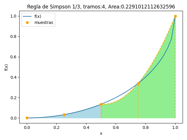
Simpson de 1/3 usa dos tramos, como se requieren al menos dos iteraciones con la fórmula se usarán 4 tramos.

h = (b-a)/4 = (1-0)/4 = 0.25

xi = [0 , 1/4, 2/4, 3/4, 1] = [0 , 1/4, 1/2, 3/4, 1]

f(x) =1 - \sqrt{ 1 - x^2}

f(0) =1 - \sqrt{ 1 - 0^2} = 0

f(1/4) =1 - \sqrt{ 1 - (1/4)^2} = 0.03175

f(1/2) =1 - \sqrt{ 1 - (1/2)^2} = 0.1339

f(3/4) =1 - \sqrt{ 1 - (3/4)^2} = 0.3385

f(1) =1 - \sqrt{ 1 - 1^2} = 1.

Area_{fx} = \frac{h}{3} (f(0)+4f(1/4)+f(1/2)) +

+ \frac{h}{3}(f(1/2)+4f(3/4)+f(1))

Area_{fx} = \frac{0.25}{3} (0+4(0.03175)+0.1339)

+ \frac{0.25}{3}(0.1339+4(0.3385)+1) = 0.2291

la cota de error de truncamiento es:

errado_truncar = -h⁵/90 = 0.00001085

errado_total = 2*errado_tramo =0.00002170

literal c.

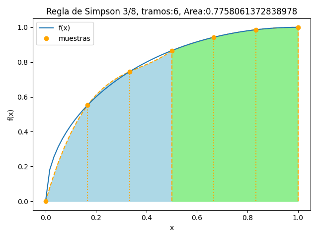
Simpson de 3/8 usa tres tramos, como se requieren al menos dos iteraciones con la fórmula se usarán 6 tramos en el intervalo [0,1].

h = (b-a)/6 = (1-0)/6 = 1/6 = 0.1666

xi = [0 , 1/6, 2/6, 3/6, 4/6, 5/6, 1] = [0 , 1/6, 1/3, 1/2, 4/6, 5/6, 1]

g(x) =\sqrt{ 1 - (x-1)^2}

g(0) =\sqrt{ 1 - (0-1)^2} =0

g(1/6) =\sqrt{ 1 - (1/6-1)^2} =0.5527

g(1/3) =\sqrt{ 1 - (1/3-1)^2}=0.7453

g(1/2) =\sqrt{ 1 - (1/2-1)^2} =0.8660

g(4/6) =\sqrt{ 1 - (4/6-1)^2} =0.9428

g(5/6) =\sqrt{ 1 - (5/6-1)^2} =0.9860

g(1) =\sqrt{ 1 - (1-1)^2} =1

Area_{gx} =\frac{3}{8}h(g(0)+3g(1/6)+3g(1/3)+g(1/2)) +

+\frac{3}{8}h(g(1/2)+3g(4/6)+3g(5/6)+g(1))

Area_{gx} =\frac{3}{8}\left(\frac{1}{6}\right)(0+3(0.5527)+3(0.7453)+0.8660) +

+\frac{3}{8}\left(\frac{1}{6}\right)(0.8660+3(0.9428)+3(0.9860)+1) =0.7758

la cota de error de truncamiento es:

errado_truncar = -3/80 h⁵ = =-3/80 (1/6)⁵ = 0.000004822

por dos iteraciones con la fórmula, el doble = 0.000009645

literal d

Area_almendra = Area_gx - Area_fx = 0.7758-0.2291 = 0.5467

el error de truncamiento se muestra en los literales anteriores.

literal e

tramos: 4
fx(xi): [0.         0.03175416 0.1339746  0.33856217 1.        ]
Integral fx con Simpson1/3:  0.2291012112632596
tramos: 6
gx(xi): [0.         0.5527708  0.74535599 0.8660254  0.94280904 0.9860133  1.        ]
Integral fx con Simpson 3/8:  0.7758061372838978

Algoritmo en Python para f(x)

# 2Eva2025PAOII_T3 Área en forma de almendra
# Regla Simpson 1/3 para f(x) entre [a,b],tramos
import numpy as np
 
# INGRESO
fx = lambda x: 1-np.sqrt(1-(x-0)**2)
a = 0 # intervalo de integración
b = 1
tramos = 2*2 # par, múltiplo de 2
 
# validar: tramos debe múltiplo de 2
while tramos%2 > 0: 
    print('tramos: ',tramos)
    tramos = int(input('tramos debe ser par: '))
 
# PROCEDIMIENTO
muestras = tramos + 1
xi = np.linspace(a,b,muestras)
fi = fx(xi)
 
# Regla de Simpson 1/3
h = (b-a)/tramos
suma = 0 # integral numérico
for i in range(0,tramos,2):
    S13= (h/3)*(fi[i]+4*fi[i+1]+fi[i+2])
    suma = suma + S13
 
# SALIDA
print('tramos:', tramos)
print('fx(xi):',fi)
print('Integral fx con Simpson1/3: ', suma)

Gráfica en Python para f(x)

# GRAFICA ---------------------
import matplotlib.pyplot as plt
 
titulo = 'Regla de Simpson 1/3'
titulo = titulo + ', tramos:'+str(tramos)
titulo = titulo + ', Area:'+str(suma)
 
fx_existe = True
try: 
    # fx suave aumentando muestras
    muestrasfxSuave = tramos*10 + 1
    xk = np.linspace(a,b,muestrasfxSuave)
    fk = fx(xk)
except NameError:
    # falta variables a,b,muestras y la función fx
    fx_existe = False
 
try: # existen mensajes de error
    msj_existe = len(msj)
except NameError:
    # falta variables mensaje: msj
    msj = []  
 
# Simpson 1/3 relleno y bordes, cada 2 tramos
for i in range(0,muestras-1,2): 
    x_tramo = xi[i:(i+2)+1]
    f_tramo = fi[i:(i+2)+1]
 
    # interpolación polinomica a*(x**2)+b*x+c
    coef = np.polyfit(x_tramo, f_tramo, 2) # [a,b,c]
    px = lambda x: coef[0]*(x**2)+coef[1]*x+coef[2]
 
    xp = np.linspace(x_tramo[0],x_tramo[-1],21)
    fp = px(xp)
     
    plt.plot(xp,fp,linestyle='dashed',color='orange')
     
    relleno = 'lightgreen'
    if (i/2)%2==0: # bloque 2 tramos, es par
        relleno ='lightblue'
    if len(msj)==0: # sin errores
        plt.fill_between(xp,fp,fp*0,color=relleno)
 
# Divisiones verticales Simpson 1/3
for i in range(0,muestras,1):
    tipolinea = 'dotted'
    if i%2==0: # i par, multiplo de 2
        tipolinea = 'dashed'
    if len(msj)==0: # sin errores
        plt.vlines(xi[i],0,fi[i],linestyle=tipolinea,
                   color='orange')
 
# Graficar f(x), puntos
if fx_existe==True:
    plt.plot(xk,fk,label='f(x)')
plt.plot(xi,fi,'o',color='orange',label ='muestras')
 
plt.xlabel('x')
plt.ylabel('f(x)')
plt.title(titulo)
plt.legend()
plt.tight_layout()
plt.show()

Algoritmo en Python para g(x)

# --------------------------------------------------
# Regla Simpson 3/8 para f(x) entre [a,b],tramos
import numpy as np
 
# INGRESO
fx = lambda x: np.sqrt(1-(x-1)**2)

a = 0 # intervalo de integración
b = 1
tramos = 3*2 # multiplo de 3
 
# validar: tramos debe ser múltiplo de 3
while tramos%3 >0:
    print('tramos: ',tramos)
    txt = 'tramos debe ser múltiplo de 3:'
    tramos = int(input(txt))
 
# PROCEDIMIENTO
muestras = tramos + 1
xi = np.linspace(a,b,muestras)
fi = fx(xi)
 
# Regla de Simpson 3/8
h = (b-a)/tramos
suma = 0 # integral numérico
for i in range(0,tramos-2,3): #muestras-3
    S38 = (3/8)*h*(fi[i]+3*fi[i+1]+3*fi[i+2]+fi[i+3])
    suma = suma + S38
 
# SALIDA
print('tramos:', tramos)
print('gx(xi):',fi)
print('Integral fx con Simpson 3/8: ', suma)

Gráfica en Python para g(x)

# GRAFICA ---------------------
import matplotlib.pyplot as plt
 
titulo = 'Regla de Simpson 3/8'
titulo = titulo + ', tramos:'+str(tramos)
titulo = titulo + ', Area:'+str(suma)
 
fx_existe = True
try: 
    # fx suave aumentando muestras
    muestrasfxSuave = tramos*10 + 1
    xk = np.linspace(a,b,muestrasfxSuave)
    fk = fx(xk)
except NameError:
    fx_existe = False
 
try: # existen mensajes de error
    msj_existe = len(msj)
except NameError:
    msj = []  
 
# Simpson 3/8 relleno y bordes, cada 3 tramos
for i in range(0,muestras-2,3):
    x_tramo = xi[i:(i+3)+1]
    f_tramo = fi[i:(i+3)+1]
 
    # interpolación polinomica a*(x**3)+b*(x**2)+c*x+d
    coef = np.polyfit(x_tramo, f_tramo, 3) # [a,b,c,d]
    px = lambda x: coef[0]*(x**3)+coef[1]*(x**2)+coef[2]*x+coef[3]
     
    xp = np.linspace(x_tramo[0],x_tramo[-1],21)
    fp = px(xp)
     
    plt.plot(xp,fp,linestyle='dashed',color='orange')
     
    relleno = 'lightgreen'
    if (i/3)%2==0: # bloque 3 tramos, es par
        relleno ='lightblue'
    plt.fill_between(xp,fp,fp*0,color=relleno)
        
# Divisiones entre Simpson 3/8
for i in range(0,muestras,1):
    tipolinea = 'dotted'
    if i%3==0: # i es multiplo de 3
        tipolinea = 'dashed'
    if len(msj)==0: # sin errores
        plt.vlines(xi[i],0,fi[i],linestyle=tipolinea,
                   color='orange')
 
# Graficar f(x), puntos
if fx_existe==True:
    plt.plot(xk,fk,label='f(x)')
plt.plot(xi,fi,'o',color='orange',label ='muestras')
 
plt.xlabel('x')
plt.ylabel('f(x)')
plt.title(titulo)
plt.legend()
plt.tight_layout()
plt.show()