s3Eva2021PAOI_T1 Tensiones en cables por carga variable

Ejercicio: 3Eva2021PAOI_T1 Tensiones en cables por carga variable

Planteamiento del problema

Las ecuaciones de equilibrio del sistema corresponden a:

-T_{CA} \cos (\alpha) + T_{CB} \cos (\beta) + P \sin (\theta) = 0

T_{CA} \sin (\alpha) + T_{CB} \sin (\beta) - P \cos (\theta) = 0

se reordenan considerando que P y θ son valores constantes para cualquier caso

T_{CA} \cos (\alpha) - T_{CB} \cos (\beta) = P \sin (\theta)

T_{CA} \sin (\alpha) + T_{CB} \sin (\beta) = P \cos (\theta)

se convierte a la forma matricial

\begin{bmatrix} \cos (\alpha) & -\cos (\beta) \\ \sin (\alpha) & \sin (\beta) \end{bmatrix} \begin{bmatrix} T_{CA} \\ T_{CB} \end{bmatrix} = \begin{bmatrix} P \sin (\theta) \\ P \cos (\theta) \end{bmatrix}

tomando valores por ejemplo:

α = 35°, β = 75°, P = 400 lb, Δθ = 5°

θ = 75-90 = -15

\begin{bmatrix} \cos (35) & -\cos (75) \\ \sin (35) & \sin (75) \end{bmatrix} \begin{bmatrix}T_{CA} \\ T_{CB} \end{bmatrix} = \begin{bmatrix} 400 \sin (-15) \\ 400 \cos (15) \end{bmatrix}

Desarrollo analítico

matriz aumentada

\begin{bmatrix} \cos (35) & - \cos (75) & 400 \sin (-15) \\ \sin (35) & \sin (75 ) & 400 \cos (15 ) \end{bmatrix}

A = 
[[ 0.81915204 -0.25881905]
 [ 0.57357644  0.96592583]]
B = 
[-103.52761804  386.37033052]

AB = 
[[ 0.81915204 -0.25881905 -103.52761804]
 [ 0.57357644  0.96592583 386.37033052]]

Pivoteo parcial por filas

cos(-15°) tendría mayor magnitud que sin(-15°), por lo que la matriz A se encuentra pivoteada

Eliminación hacia adelante

pivote =  0.81915204/0.57357644
[[ 0.81915204 -0.25881905 -103.52761804]
 [ 0.0         1.63830408  655.32162903]]

Sustitución hacia atrás

usando la última fila:

1.63830408 T_CB = 655.32162903
T_CB = 400

luego la primera fila:

0.81915204T_CA -0.25881905T_CB = -103.52761804

0.81915204T_CA = 0.25881905T_CB -103.52761804

T_CA = 2,392 x10^-6 ≈ 0

Se deja como tarea realizar el cálculo para: θ+Δθ

Instrucciones en Python

Resultado:

Resultado: [TCA, TCB], diferencia 
[array([3.46965006e-14, 4.00000000e+02]), -399.99999999999994]

usando el intervalo para θ₁ y θ₂:

Algoritmo con Python

con las instrucciones:

import numpy as np
import matplotlib.pyplot as plt

# Tema 1
def funcion(P,theta,alfa,beta):
    # ecuaciones
    A = np.array([[np.cos(alfa), -np.cos(beta)],
                  [np.sin(alfa),  np.sin(beta)]])
    B = np.array([P*np.sin(theta), P*np.cos(theta)])

    # usar un algoritmo directo
    X = np.linalg.solve(A,B)
    
    diferencia = X[0]-X[1]
    return([X,diferencia])    

# INGRESO
alfa = np.radians(35)
beta = np.radians(75)
P = 400

# PROCEDIMIENTO
theta = beta-np.radians(90)
resultado = funcion(P,theta,alfa, beta)

# SALIDA
print("Resultado: [TCA, TCB], diferencia")
print(resultado)

# Tema 1b --------------
# PROCEDIMIENTO
dtheta = np.radians(5)
theta1 = beta-np.radians(90)
theta2 = np.radians(90)-alfa

tabla = []
theta = theta1
while not(theta>=theta2):
    X = funcion(P,theta,alfa,beta)[0] # usa vector X
    tabla.append([theta,X[0],X[1]])
    theta = theta + dtheta
    
tabla = np.array(tabla)
thetai = np.degrees(tabla[:,0])
Tca = tabla[:,1]
Tcb = tabla[:,2]

# SALIDA
print('tetha, TCA, TCB')
print(tabla)

# Grafica
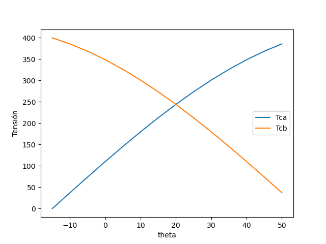
plt.plot(thetai,Tca, label='Tca')
plt.plot(thetai,Tcb, label='Tcb')
# plt.axvline(np.degrees(c))
plt.legend()
plt.xlabel('theta')
plt.ylabel('Tensión')
plt.show()