Ejercicio: 3Eva_IT2010_T1 Ecuación Verhulst
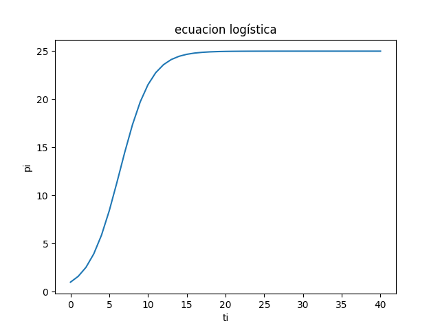
Para probar el ejercico se usa po=1, a=0.5 b=0.02 y tiempo maximo = 40
con el algoritmo se puede observar:
poblacion inicial p0:1
factor a:0.5
factor b:0.02
calcular en t:40
tiempo:
[0, 1, 2, 3, 4, 5, 6, 7, 8, 9, 10, 11, 12, 13, 14, 15, 16, 17, 18, 19, 20, 21, 22, 23, 24, 25, 26, 27, 28, 29, 30, 31, 32, 33, 34, 35, 36, 37, 38, 39, 40]
pi:
[1.0, 1.6070209244539886, 2.5434661610272977, 3.9338336459524355, 5.885057578381894, 8.417395145518748, 11.39009430586252, 14.494961881174662, 17.366232541771218, 19.73763290519436, 21.51998720327935, 22.766959376324014, 23.596257413785583, 24.129351687331045, 24.464588393188883, 24.67249666532522, 24.80032998711217, 24.878512232622807, 24.92617278160938, 24.95516943765841, 24.972789690449925, 24.983489042065916, 24.98998299475044, 24.99392342119231, 24.996314016127226, 24.99776420806526, 24.998643875922703, 24.999177451612496, 24.999501092725076, 24.99969739506529, 24.999816459955184, 24.999888677013956, 24.999932479077533, 24.999959046446833, 24.999975160398368, 24.999984934014144, 24.999990862015494, 24.99999445753143, 24.99999663832259, 24.999997961039472, 24.99999876330789]
>>>
que produce la siguiente gráfica
Instrucciones en Python
# 3Eva_IT2010_T1 Ecuación Verhulst
import numpy as np
import matplotlib.pyplot as plt

def f_logistica(p0,a,b,t):
    numerador = a*p0
    denominador = b*p0+(a-b*p0)*np.exp(-a*t)
    p = numerador/denominador
    return(p)

# PROGRAMA ------
# INGRESO
p0 = float(input("poblacion inicial p0:"))
a  = float(input("factor a:"))
b  = float(input("factor b:"))
t  = float(input("calcular en t:"))

# PROCEDIMIENTO
ti = []
pi = []
i = 0
while i<=t:
    pi.append(f_logistica(p0,a,b,i))
    ti.append(i)
    i = i + 1

# SALIDA
np.set_printoptions(precision=3)
print('tiempo:')
print(ti)
print('pi:')
print(pi)

# grafica
plt.plot(ti,pi)
plt.xlabel('ti')
plt.ylabel('pi')
plt.title('ecuacion logística')
plt.show()
Tarea, estimar el tiempo t cuando la población se duplica