s2Eva_IT2010_T2 Movimiento angular

Ejercicio: 2Eva_IT2010_T2 Movimiento angular

Para resolver, se usa Runge-Kutta_fg de segundo orden como ejemplo

y'' + 10 \sin (y) =0

se hace

y' = z = f(t,y,z)

y se estandariza:

y'' =z'= -10 \sin (y) = g(t,y,z)

teniendo como punto de partida t₀=0, y₀=0 y z₀=0.1

y(0)=0, y'(0)=0.1

Se desarrolla el algotitmo para obtener los valores:

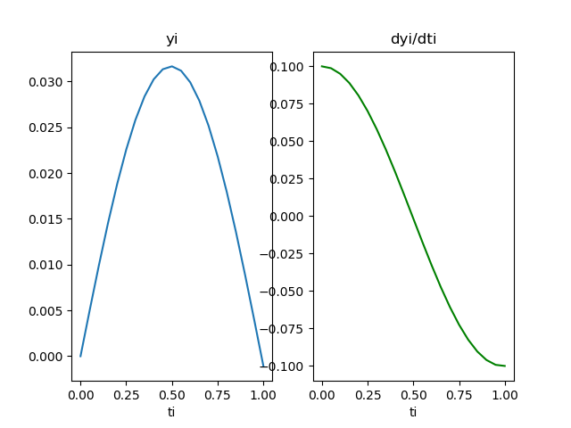
 [ t, 		 y, 	 dyi/dti=z]
[[ 0.          0.          0.1       ]
 [ 0.2         0.02        0.08000133]
 [ 0.4         0.03200053  0.02401018]
 [ 0.6         0.03040355 -0.04477916]
 [ 0.8         0.01536795 -0.09662411]
 [ 1.         -0.00703034 -0.10803459]]

que permiten generar la gráfica de respuesta:

---

Algoritmo en Python

# 2Eva_IT2010_T2 Movimiento angular
import numpy as np
import matplotlib.pyplot as plt

def rungekutta2_fg(f,g,x0,y0,z0,h,muestras):
    tamano = muestras + 1
    estimado = np.zeros(shape=(tamano,3),dtype=float)
    # incluye el punto [x0,y0,z0]
    estimado[0] = [x0,y0,z0]
    xi = x0
    yi = y0
    zi = z0
    for i in range(1,tamano,1):
        K1y = h * f(xi,yi,zi)
        K1z = h * g(xi,yi,zi)
        
        K2y = h * f(xi+h, yi + K1y, zi + K1z)
        K2z = h * g(xi+h, yi + K1y, zi + K1z)

        yi = yi + (K1y+K2y)/2
        zi = zi + (K1z+K2z)/2
        xi = xi + h
        
        estimado[i] = [xi,yi,zi]
    return(estimado)

# INGRESO theta = y
ft = lambda t,y,z: z
gt = lambda t,y,z: -10*np.sin(y)

t0 = 0
y0 = 0
z0 = 0.1
h=0.2
muestras = 5

# PROCEDIMIENTO
tabla = rungekutta2_fg(ft,gt,t0,y0,z0,h,muestras)

# SALIDA
print(' [ t, \t\t y, \t dyi/dti=z]')
print(tabla)

# Grafica
ti = np.copy(tabla[:,0])
yi = np.copy(tabla[:,1])
zi = np.copy(tabla[:,2])
plt.subplot(121)
plt.plot(ti,yi)
plt.xlabel('ti')
plt.title('yi')
plt.subplot(122)
plt.plot(ti,zi, color='green')
plt.xlabel('ti')
plt.title('dyi/dti')
plt.show()