Ejercicio: 2Eva_IIT2018_T2 Kunge Kutta 2do Orden x»
\frac{\delta ^2 x}{\delta t^2} + 5t\frac{\delta x}{\delta t} +(t+7)\sin (\pi t) = 0 x'' + 5tx' +(t+7)\sin (\pi t) = 0 x'' = -5tx' +(t+7)\sin (\pi t) = 0si se usa z=x’
z' = -5tz +(t+7)\sin (\pi t) = 0se convierte en:
f(t,x,z) = x’ = z
g(t,x,z) = x» = z’ = -5tz +(t+7)sin (π t) = 0
Donde se aplica el algoritmo de Runge Kutta
http://blog.espol.edu.ec/analisisnumerico/8-2-2-runge-kutta-d2y-dx2/
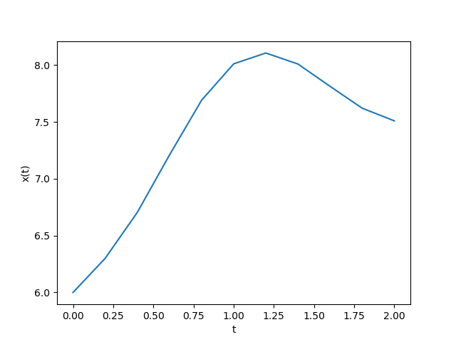
   t,              x,              z
[[ 0.00000000e+00  6.00000000e+00  1.50000000e+00]
 [ 2.00000000e-01  6.30000000e+00  1.77320538e+00]
 [ 4.00000000e-01  6.70381805e+00  2.26987703e+00]
 [ 6.00000000e-01  7.20775473e+00  2.41163944e+00]
 [ 8.00000000e-01  7.68994485e+00  1.90531839e+00]
 [ 1.00000000e+00  8.01027755e+00  9.52659193e-01]
 [ 1.20000000e+00  8.10554347e+00 -5.65431040e-03]
 [ 1.40000000e+00  8.00869435e+00 -6.09147239e-01]
 [ 1.60000000e+00  7.81236802e+00 -7.16247408e-01]
 [ 1.80000000e+00  7.62013640e+00 -3.92947221e-01]
 [ 2.00000000e+00  7.50882725e+00  1.63598524e-01]]
Instrucciones en Python
# 2Eva_IIT2018_T2 Kunge Kutta 2do Orden x''
import numpy as np

def rungekutta2_fg(f,g,x0,y0,z0,h,muestras):
    tamano = muestras + 1
    estimado = np.zeros(shape=(tamano,3),dtype=float)
    # incluye el punto [x0,y0]
    estimado[0] = [x0,y0,z0]
    xi = x0
    yi = y0
    zi = z0
    for i in range(1,tamano,1):
        K1y = h * f(xi,yi,zi)
        K1z = h * g(xi,yi,zi)

        K2y = h * f(xi+h, yi + K1y, zi + K1z)
        K2z = h * g(xi+h, yi + K1y, zi + K1z)

        yi = yi + (K1y+K2y)/2
        zi = zi + (K1z+K2z)/2
        xi = xi + h

        estimado[i] = [xi,yi,zi]
    return(estimado)

# PROGRAMA
# INGRESO
f = lambda t,x,z: z
g = lambda t,x,z: -5*t*z+(t+7)*np.sin(np.pi*t)
t0 = 0
x0 = 6
z0 = 1.5
h = 0.2
muestras = 10

# PROCEDIMIENTO
tabla = rungekutta2_fg(f,g,t0,x0,z0,h,muestras)

# SALIDA
print(tabla)
# GRAFICA
import matplotlib.pyplot as plt
plt.plot(tabla[:,0],tabla[:,1])
plt.xlabel('t')
plt.ylabel('x(t)')
plt.show()