
Ejercicio: 2Eva_IIT2019_T2 EDO, problema de valor inicial
la ecuación del problema planteado es:
y'(t) = f(t,y) = \frac{y}{2t^3}0 ≤ t ≤ 1
y(0.5) = 1.5
literal a
La solución empieza usando la Serie de Taylor por ejemplo para tres términos:
y_{i+1} = y_{i} + h y'_i + \frac{h^2}{2!} y''_i x_{i+1} = x_{i} + h E = \frac{h^3}{3!} y'''(z) = O(h^3)Se observa que se tiene el valor inicial y la primera derivada, si usamos tres términos se puede usar la segunda derivada.
y'(t) = f(t,y) = \frac{y}{2t^3} y''(t) = f'(t,y) = \frac{y'}{2t^3} + y \Big(\frac{-3}{2t^4}\Big) y''(t) = \frac{1}{2t^3}\Big( \frac{y}{2t^3} \Big) - \frac{3y}{2t^4} y''(t) = \frac{y}{4t^6} -\frac{3y}{2t^4}por lo que la ecuación de Taylor a usar queda de la siguiente forma:
y_{i+1} = y_{i} + h y'_i + \frac{h^2}{2!} y''_i y_{i+1} = y_{i} + h\frac{y}{2t^3}+\frac{h^2}{2} \Big( \frac{y}{4t^6} -\frac{3y}{2t^4}\Big)que es la ecuacion que se usará con un error de O(h3)
Reemplazando los valores en la fórmula se obtiene la siguiente tabla:
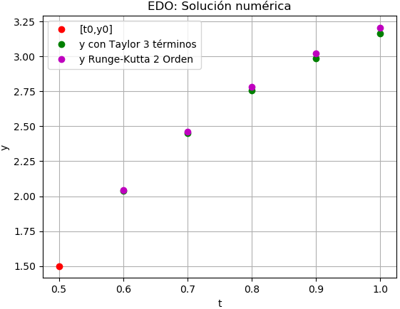
estimado
 [ti,      yi,      d1yi,    d2yi]
[[  0.5    1.5      6.      -12.        ]
 [  0.6    2.04     4.7222  -12.68004115]
 [  0.7    2.4488   3.5697  -10.09510219]
 [  0.8    2.7553   2.6907  -7.46259891]
 [  0.9    2.9870   2.0487  -5.42399041]
 [  1.     3.1648   0.       0.        ]]
cuya gráfica es:
literal b
Para desarrollar Runge-Kutta de 2do orden se dispone de los siguientes datos:
y'(t) = f(t,y) = \frac{y}{2t^3}t0 = 0.5, y0 = 1.5, h = 0.1
pasos del algoritmo,
K_1 = h * y'(t_i) K_2 = h * y'(t_i+h, y_i + K_1) y_{i+1} = y_i + \frac{K_1+K_2}{2} t_i = t_i + h</p> <p>iteración 1: i = 0
K_1 = 0.1 * y'(0.5) = 0.6 K_2 = 0.1 * y'(0.5+0.1, 1.5 + 0.6) = 0.4861 y_{1} = 1.5 + \frac{0.6+0.4861}{2} = 2.0430 t_1 = 0.5 + 0.1 = 0.6</p> <p>iteración 2: i = 1
K_1 = 0.1 * y'(0.6) = 0.4729 K_2 = 0.1 * y'(0.6+0.1, 2.0430 + 0.4729) = 0.3667 y_{1} = 2.0430 + \frac{0.4729+0.3667}{2} = 2.4629 t_1 = 0.6 + 0.1 = 0.7</p> <p>iteración 3: i = 2
K_1 = 0.1 * y'(0.7) = 0.3590 K_2 = 0.1 * y'(0.7+0.1, 2.4629 + 0.3590) = 0.3667 y_{1} = 2.4629 + \frac{0.3590+0.3667}{2} = 2.7802 t_1 = 0.7 + 0.1 = 0.8</p> <p>obteniendo la siguiente tabla:
estimado
 [ti,   yi,     K1,     K2]
[[0.5   1.5     0.      0.    ]
 [0.6   2.0430  0.6     0.4861]
 [0.7   2.4629  0.4729  0.3667]
 [0.8   2.7802  0.3590  0.2755]
 [0.9   3.0206  0.2715  0.2093]
 [1.    3.2048  0.2071  0.1613]]
Diferencias entre Taylor y Runge-Kutta2
[ 0.   -0.0030 -0.0140 -0.0248 -0.0335 -0.0400]
Algoritmo en Python
# EDO. Método de Taylor 3 términos
# Runge-Kutta de 2 Orden
# 2Eva_IIT2019_T2 EDO, problema de valor inicial
import numpy as np

# Funciones desarrolladas en clase
def edo_taylor3t(d1y,d2y,x0,y0,h,muestras):
    tamano = muestras + 1
    estimado = np.zeros(shape=(tamano,4),dtype=float)
    # incluye el punto [x0,y0]
    estimado[0] = [x0,y0,0,0]
    x = x0
    y = y0
    for i in range(1,tamano,1):
        estimado[i-1,2:]= [d1y(x,y),d2y(x,y)]
        y = y + h*d1y(x,y) + ((h**2)/2)*d2y(x,y)
        x = x+h
        estimado[i,0:2] = [x,y]
    return(estimado)
def rungekutta2(d1y,x0,y0,h,muestras):
    tamano = muestras + 1
    estimado = np.zeros(shape=(tamano,4),dtype=float)
    # incluye el punto [x0,y0]
    estimado[0] = [x0,y0,0,0]
    xi = x0
    yi = y0
    for i in range(1,tamano,1):
        K1 = h * d1y(xi,yi)
        K2 = h * d1y(xi+h, yi + K1)
        yi = yi + (K1+K2)/2
        xi = xi + h
        estimado[i] = [xi,yi,K1,K2]
    return(estimado)

# PROGRAMA PRUEBA
# INGRESO
# d1y = y', d2y = y''
d1y = lambda t,y: y/(2*t**3)
d2y = lambda t,y: y/(4*t**6)-(3/2)*y/(t**4)
t0 = 0.5
y0 = 1.5
h = 0.1
muestras = 5

# PROCEDIMIENTO
# Edo con Taylor
puntos = edo_taylor3t(d1y,d2y,t0,y0,h,muestras)
ti = puntos[:,0]
yi = puntos[:,1]

# Runge-Kutta
puntosRK2 = rungekutta2(d1y,t0,y0,h,muestras)
# ti = puntosRK2[:,0] # lo mismo del anterior
yiRK2 = puntosRK2[:,1]

# diferencias
diferencia = yi-yiRK2

# SALIDA
print('estimado[ti, yi, d1yi, d2yi]')
print(puntos)

print('estimado[ti, yi, K1, K2]')
print(puntosRK2)

print('Diferencias entre Taylor y Runge-Kutta2')
print(diferencia)

# Gráfica
import matplotlib.pyplot as plt
plt.plot(ti[0],yi[0],'o', color='r',
         label ='[t0,y0]')
plt.plot(ti[1:],yi[1:],'o', color='g',
         label ='y con Taylor 3 términos')
plt.plot(ti[1:],yiRK2[1:],'o', color='m',
         label ='y Runge-Kutta 2 Orden')
plt.title('EDO: Solución numérica')
plt.xlabel('t')
plt.ylabel('y')
plt.legend()
plt.grid()
plt.show())