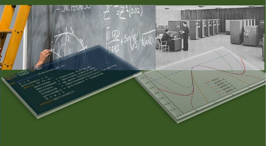
Ejercicio: 2Eva_IT2012_T3_MN EDO Taylor 2 Contaminación de estanque
La ecuación a resolver con Taylor es:
s'- \frac{26s}{200-t} - \frac{5}{2} = 0Para lo que se plantea usar la primera derivada:
s'= \frac{26s}{200-t}+\frac{5}{2}con valores iniciales de s(0) = 0, h=0.1
La fórmula de Taylor para tres términos es:
s_{i+1}= s_{i}+s'_{i}h + \frac{s''_{i}}{2}h^2 + errorPara el desarrollo se compara la solución con dos términos, tres términos y Runge Kutta.
1. Solución con dos términos de Taylor
Iteraciones
i = 0, t0 = 0, s(0)=0
s'_{0}= \frac{26s_{0}}{200-t_{0}}+\frac{5}{2} = \frac{26(0)}{200-0}+\frac{5}{2} = \frac{5}{2} s_{1}= s_{0}+s'_{0}h = 0+ \frac{5}{2}*0.1= 0.25t1 = t0+h = 0+0.1 = 0.1
i=1
s'_{1}= \frac{26s_{1}}{200-t_{1}}+\frac{5}{2} = \frac{26(0.25)}{200-0.1}+\frac{5}{2} = 2.5325 s_{2}= s_{1}+s'_{1}h = 0.25 + (2.5325)*0.1 = 0.5032
t2 = t1+h = 0.1+0.1 = 0.2
i=2,
resolver como tarea
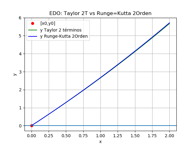
2. Resolviendo con Python
estimado
 [xi,yi Taylor,yi Runge-Kutta, diferencias]
[[ 0.0  0.0000e+00  0.0000e+00  0.0000e+00]
 [ 0.1  2.5000e-01  2.5163e-01 -1.6258e-03]
 [ 0.2  5.0325e-01  5.0655e-01 -3.2957e-03]
 [ 0.3  7.5980e-01  7.6481e-01 -5.0106e-03]
 [ 0.4  1.0197e+00  1.0265e+00 -6.7714e-03]
 [ 0.5  1.2830e+00  1.2916e+00 -8.5792e-03]
 [ 0.6  1.5497e+00  1.5601e+00 -1.0435e-02]
 [ 0.7  1.8199e+00  1.8322e+00 -1.2339e-02]
 [ 0.8  2.0936e+00  2.1079e+00 -1.4294e-02]
 [ 0.9  2.3710e+00  2.3873e+00 -1.6299e-02]
 [ 1.0  2.6519e+00  2.6703e+00 -1.8357e-02]
 [ 1.1  2.9366e+00  2.9570e+00 -2.0467e-02]
 [ 1.2  3.2250e+00  3.2476e+00 -2.2632e-02]
 [ 1.3  3.5171e+00  3.5420e+00 -2.4853e-02]
 [ 1.4  3.8132e+00  3.8403e+00 -2.7129e-02]
 [ 1.5  4.1131e+00  4.1426e+00 -2.9464e-02]
 [ 1.6  4.4170e+00  4.4488e+00 -3.1857e-02]
 [ 1.7  4.7248e+00  4.7592e+00 -3.4310e-02]
 [ 1.8  5.0368e+00  5.0736e+00 -3.6825e-02]
 [ 1.9  5.3529e+00  5.3923e+00 -3.9402e-02]
 [ 2.0  5.6731e+00  5.7152e+00 -4.2043e-02]]
error en rango:  0.04204310894163932
2. Algoritmo en Python
# EDO. Método de Taylor 3 términos
# estima la solucion para muestras espaciadas h en eje x
# valores iniciales x0,y0
# entrega arreglo [[x,y]]
import numpy as np

def edo_taylor2t(d1y,x0,y0,h,muestras):
    tamano = muestras + 1
    estimado = np.zeros(shape=(tamano,2),dtype=float)
    # incluye el punto [x0,y0]
    estimado[0] = [x0,y0]
    x = x0
    y = y0
    for i in range(1,tamano,1):
        y = y + h*d1y(x,y) # + ((h**2)/2)*d2y(x,y)
        x = x+h
        estimado[i] = [x,y]
    return(estimado)

def rungekutta2(d1y,x0,y0,h,muestras):
    tamano = muestras + 1
    estimado = np.zeros(shape=(tamano,2),dtype=float)
    # incluye el punto [x0,y0]
    estimado[0] = [x0,y0]
    xi = x0
    yi = y0
    for i in range(1,tamano,1):
        K1 = h * d1y(xi,yi)
        K2 = h * d1y(xi+h, yi + K1)

        yi = yi + (K1+K2)/2
        xi = xi + h

        estimado[i] = [xi,yi]
    return(estimado)

# PROGRAMA PRUEBA
# 2Eva_IIT2016_T3_MN EDO Taylor 2, Tanque de agua

# INGRESO.
# d1y = y' = f, d2y = y'' = f'
d1y = lambda x,y: 26*y/(200-x)+5/2
x0 = 0
y0 = 0
h = 0.1
muestras = 20

# PROCEDIMIENTO
puntos = edo_taylor2t(d1y,x0,y0,h,muestras)
xi = puntos[:,0]
yi = puntos[:,1]

# Con Runge Kutta
puntosRK2 = rungekutta2(d1y,x0,y0,h,muestras)
xiRK2 = puntosRK2[:,0]
yiRK2 = puntosRK2[:,1]

# diferencias
diferencias = yi-yiRK2
error = np.max(np.abs(diferencias))
tabla = np.copy(puntos)
tabla = np.concatenate((puntos,np.transpose([yiRK2]),
                        np.transpose([diferencias])),
                       axis = 1)

# SALIDA
np.set_printoptions(precision=4)
print('estimado[xi,yi Taylor,yi Runge-Kutta, diferencias]')
print(tabla)
print('error en rango: ', error)

# Gráfica
import matplotlib.pyplot as plt
plt.plot(xi[0],yi[0],'o',
         color='r', label ='[x0,y0]')
plt.plot(xi[0:],yi[0:],'-',
         color='g',
         label ='y Taylor 2 términos')
plt.plot(xiRK2[0:],yiRK2[0:],'-',
         color='blue',
         label ='y Runge-Kutta 2Orden')
plt.axhline(y0/2)
plt.title('EDO: Taylor 2T vs Runge=Kutta 2Orden')
plt.xlabel('x')
plt.ylabel('y')
plt.legend()
plt.grid()
plt.show()
Usando Taylor con 3 términos
estimado
 [xi,        yi,        d1yi,      d2yi      ]
[[0.         0.         2.5        0.325     ]
 [0.1        0.251625   2.53272761 0.32958302]
 [0.2        0.50654568 2.56591685 0.33423301]
 [0.3        0.76480853 2.59957447 0.33895098]
 [0.4        1.02646073 2.63370731 0.34373796]
 [0.5        1.29155015 2.66832233 0.348595  ]
 [0.6        1.56012536 2.70342658 0.35352316]
 [0.7        1.83223563 2.73902723 0.35852351]
 [0.8        2.10793097 2.77513155 0.36359715]
 [0.9        2.38726211 2.81174694 0.36874519]
 [1.         2.67028053 2.84888087 0.37396876]
 [1.1        2.95703846 2.88654098 0.37926901]
 [1.2        3.24758891 2.92473497 0.3846471 ]
 [1.3        3.54198564 2.96347069 0.39010422]
 [1.4        3.84028323 3.00275611 0.39564157]
 [1.5        4.14253705 3.04259931 0.40126036]
 [1.6        4.44880328 3.08300849 0.40696184]
 [1.7        4.75913894 3.12399199 0.41274727]
 [1.8        5.07360187 3.16555827 0.41861793]
 [1.9        5.39225079 3.2077159  0.42457511]
 [2.         5.71514526 0.         0.        ]]