Ejercicio: 2Eva_IT2019_T2 Péndulo vertical
Para resolver la ecuación usando Runge-Kutta se estandariza la ecuación a la forma:
\frac{d^2\theta }{dt^2}+\frac{g}{L}\sin (\theta)=0 \frac{d^2\theta }{dt^2}= -\frac{g}{L}\sin (\theta)Se simplifica su forma a:
\frac{d\theta}{dt}=z = f_t(t,\theta,z) \frac{d^2\theta }{dt^2}= z' =-\frac{g}{L}\sin (\theta) = g_t(t,\theta,z)y se usan los valores iniciales para iniciar la tabla:
\theta(0) = \frac{\pi}{6} \theta '(0) = 0| ti | θ(ti) | θ'(ti)=z |
| 0 | π/6 = 0.5235 | 0 |
| 0.2 | 0.3602 | -1.6333 |
| 0.4 | -0.0815 | -2.2639 |
| … |
para las iteraciones se usan los valores (-g/L) = (-9.8/0.6)
Iteración 1: ti = 0 ; yi = π/6 ; zi = 0
K1y = h * ft(ti,yi,zi)
    = 0.2*(0) = 0
K1z = h * gt(ti,yi,zi)
    = 0.2*(-9.8/0.6)*sin(π/6) = -1.6333

K2y = h * ft(ti+h, yi + K1y, zi + K1z)
    = 0.2*(0-1.6333)= -0.3266
K2z = h * gt(ti+h, yi + K1y, zi + K1z)
    = 0.2*(-9.8/0.6)*sin(π/6+0) = -1.6333

yi = yi + (K1y+K2y)/2
   = π/6+ (0+(-0.3266))/2 = 0.3602
zi = zi + (K1z+K2z)/2
   = 0+(-1.6333-1.6333)/2 = -1.6333
ti = ti + h = 0 + 0.2 = 0.2

estimado[i] = [0.2,0.3602,-1.6333]
Iteración 2: ti = 0.2 ; yi = 0.3602 ; zi = -1.6333
K1y = 0.2*( -1.6333) = -0.3266
K1z = 0.2*(-9.8/0.6)*sin(0.3602) = -1.1515

K2y = 0.2*(-1.6333-0.3266)= -0.5569
K2z = 0.2*(-9.8/0.6)*sin(0.3602-0.3266) = -0.1097

yi = 0.3602 + ( -0.3266 + (-0.3919))/2 = -0.0815
zi = -1.6333+(-1.151-0.1097)/2 = -2.2639
ti = ti + h = 0.2 + 0.2 = 0.4

estimado[i] = [0.4,-0.0815,-2.2639]
Se continúan con las iteraciones, hasta completar la tabla.
Tarea: realizar la Iteración 3
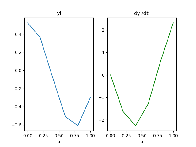
Usando el algoritmo RungeKutta_fg se obtienen los valores y luego la gráfica
 [ t, 		 y, 	 dyi/dti=z]
[[ 0.          0.52359878  0.        ]
 [ 0.2         0.36026544 -1.63333333]
 [ 0.4        -0.08155862 -2.263988  ]
 [ 0.6        -0.50774327 -1.2990876 ]
 [ 0.8        -0.60873334  0.62920692]
 [ 1.         -0.29609456  2.32161986]]
si se mejora la resolución disminuyendo h = 0.05 y muestras = 20 para cubrir el dominio [0,1] se obtiene el siguiente resultado:

Tarea: Para el literal b, se debe considerar que los errores se calculan con
Runge-Kutta 2do Orden tiene error de truncamiento O(h3)
Runge-Kutta 4do Orden tiene error de truncamiento O(h5)
Algoritmo en Python
# 3Eva_IT2019_T2 Péndulo vertical
import numpy as np
import matplotlib.pyplot as plt

def rungekutta2_fg(f,g,x0,y0,z0,h,muestras):
    tamano = muestras + 1
    estimado = np.zeros(shape=(tamano,3),dtype=float)
    # incluye el punto [x0,y0,z0]
    estimado[0] = [x0,y0,z0]
    xi = x0
    yi = y0
    zi = z0
    for i in range(1,tamano,1):
        K1y = h * f(xi,yi,zi)
        K1z = h * g(xi,yi,zi)

        K2y = h * f(xi+h, yi + K1y, zi + K1z)
        K2z = h * g(xi+h, yi + K1y, zi + K1z)

        yi = yi + (K1y+K2y)/2
        zi = zi + (K1z+K2z)/2
        xi = xi + h

        estimado[i] = [xi,yi,zi]
    return(estimado)

# INGRESO theta = y
g = 9.8
L  = 0.6
ft = lambda t,y,z: z
gt = lambda t,y,z: (-g/L)*np.sin(y)

t0 = 0
y0 = np.pi/6
z0 = 0
h=0.2
muestras = 5

# PROCEDIMIENTO
tabla = rungekutta2_fg(ft,gt,t0,y0,z0,h,muestras)

# SALIDA
print(' [ t, \t\t y, \t dyi/dti=z]')
print(tabla)

# Grafica
ti = np.copy(tabla[:,0])
yi = np.copy(tabla[:,1])
zi = np.copy(tabla[:,2])
plt.subplot(121)
plt.plot(ti,yi)
plt.xlabel('ti')
plt.title('yi')
plt.subplot(122)
plt.plot(ti,zi, color='green')
plt.xlabel('ti')
plt.title('dyi/dti')
plt.show()
Otra solución propuesta puede seguir el problema semejante: